OSI Model

Layer 7 : The Application Layer

It enables a user whether a human or software to access the network. It provides user interface and support for services such as e-mail, remote file access and transfer share database management, and other types of distributed information services.

The application layer is responsible for providing services to the user.
Provides a set of interfaces for applications to use to gain access to networked services.

Specific services of application layer include the following :

 

Network virtual terminal : A network virtual terminal is a software version of a physical terminal, and it allows a user to log on to a remote host. To do so, the application creates a software emulation of a terminal at the remote host. The user’s computer talks to the software terminal which, in turn, talks to the host, and vice versa. The remote host believes it is communicating with one of its own terminals and allows the user to log on.

File transfer, access, and management : The application allows the user to access files in a remote host (to make changes or read data), to retrieve files from a remote computer for use in the local computer, and to manage or control files in a remote computer locally.

Mail services : The application provides the basis for e-mail forwarding and storage.

Directory services : This application provides distributed database source and access for global information about various objects and services.

Layer 6 : The Presentation Layer

The Presentation layer manages data-format information for networked communications. Also called the network’s translator, it converts outgoing messages into a generic format that can be transmitted across a network; then, it converts incoming messages from that generic format into one that makes sense to the receiving application. This layer is also responsible for protocol conversion, data encryption and decryption, and graphics commands. Information sent by the Presentation layer may sometimes be compressed to reduce the amount of data to be transferred.
The presentation layer is concern with the syntax and semantics of the information exchanged between two systems. 
The presentation layer Converts data into a generic format for network transmission; for incoming messages, it converts data from this format into a format that the receiving application can understand.

Specific responsibilities of the presentation layer include following.

 

>Translation :

The presentation layer at the sender changes the information from its sender-dependent format into a common format. The presentation layer at the receiving machine changes the common format into its receiver-dependent format.

Encryption : Encryption means that the sender transforms the original information to another form and sends the resulting message out over the network. Decryption reverses the original process to transform the message into its original form.

 

Compression : Data compression reduces the number of bits contained in the information. Data compression becomes particularly important in the transmission of multimedia such as text, audio and video.

 

Layer 5 : The Session Layer 

The Session layer allows two networked resources to hold ongoing communications, called a session, across a network. In other words, applications on each end of the session are able to exchange data for the duration of the session.
The session layer is the network dialogue  controller. It establishes maintenance and synchronized the interaction between the communication devices. 
Session layer Enables two parties to hold ongoing communications—called sessions—across a network.
Specific responsibilities of the session layer include following :

 

Dialogue control : The session layer allows two systems to enter into a dialog. It allows the  communication between two processes to take place in either half-duplex or full-duplex mode.

 

Synchronization : The session layer allows a process to add check points, or  synchronization points, to a stream of data.

 

Layer 4 : The Transport Layer 

The Transport layer manages the flow control of data between parties across a network. It does layer this by segmenting long streams of data into chunks that adhere to the maximum packet size for the networking medium in use. The layer also provides error checks to guarantee error-free data delivery, and resequences chunks back into the original data when it is received. In addition, the large Transport layer provides acknowledgement of successful transmissions and is responsible for requesting retransmission if some packets do not arrive error-free.
The transport layer is final responsible for process-to-process delivery of the entire message. The process is an application program running on the host. 
Transport layer Manages the transmission of data across a network. 
Other responsibilities of the transport layer include the following :

 

Source-point addressing :Computers often run several programs at the same time. For the reason, source-to-destination delivery means delivery not only from one computer to the next  but also from specific process (running program) on one computer to a specific process (running  program) on the other. The transport layer header must therefore include a type of address called a send service-point address (or port address).

 

Segmentation and Reassembly : A message is divided into transmittable segments, with each segment connecting a sequence number. These numbers enable the transport layer to reassemble the message correctly upon arriving at the destination and to identify and replace packets that were lost in transmission.

 

Connection control : The transport layer can be either connectionless or connection-oriented. A connectionless transport layer treats each segment as an independent packet and delivers it to the transport layer at the destination machine. A connection-oriented transport layer makes a connection with the transport layer at the destination machine first before delivering the packets. After all the data are transferred, the connection is terminated.

 

Flow control : Like the data link layer, the transport layer is responsible for flow control.  However, flow control at this layer is performed end to end rather than across a single link.

 

Error control : Like the data link layer, the transport layer is responsible for error control. The sensing transport layer makes sure that the entire message arrives at the receiving transport layer without error (damage, loss, or duplication). Error correction is usually achieved through retransmission.

 

Layer 3 : The Network Layer 

The Network layer addresses messages for delivery, and translates logical network addresses and names into their physical equivalents. This layer also decides how to route transmissions between cog computers. To decide how to get data from one point to the next, the Network layer considers other al factors, such as quality of service information, alternative routes, and delivery priorities. This layer also handles packet switching, data routing, and network congestion control.
The network layer is responsible for the delivery of individual packets from the source host to the the destination host.
Network layer Handles addressing messages for delivery, as well as translates logical network addresses and names into their physical counterparts.
If two systems are connected to the same link, there is usually no need for a network layer. or However, if the two systems are attached to different networks (links) with connecting devices the between the networks (links), there is often a need for the network layer to accomplish source-to destination delivery.
Other responsibilities of the network layer include the following :

Logical addressing : The network layer adds a header to the packet coming from the upper layer that, among other things, includes the logical address of the sender and receiver which help to  distinguish the source and destination systems.

 

Routing : When independent networks or links are connected to create internet works or a for large network, the connecting devices (called routers or switches) route or switch the packets to their is final destination. One of the functions of the network layer is to provide this mechanism.

Layer 2 : The Data Link Layer 

The Data Link layer handles special data frames between the Network and Physical layers. At the receiving end, this layer packages raw data from the Physical layer into data frames for delivery to the Network layer. A data frame is the basic unit for network traffic as data is sent across the network medium; the data frame is a highly structured format in which data from upper layers is placed for sending, and from which data from upper layers is taken on receipt.
The data link layer is responsible for moving frames from one hop (node) to the next. 
Data Link layer Sends special data frames from the Network layer to the Physical layer.

Other responsibilities of the data link layer include the following.

Framing : The data link layer divides the stream of bits received from the network layer into manageable data units called frames.
Physical addressing : If frames are to be distributed to different systems on the network, the data link layer adds a header to the frame to define the sender and/or receiver or the frame. If the frame is intended for a system outside the sender’s network, the receiver address is the address of the device that connects the network to next one.
Flow control : If the rate at which data are absorbed by the receiver is less then the rate at which data are produced in the sender, the data link layer imposes a flow control mechanism to avoid overwhelming the receiver.
Error control : The data link layer adds reliability to the physical layer by adding mechanism to detect and retransmit damaged or lost frames. It also uses a mechanism to recognize duplicate frames. Error control is normally achieved through a trailer added to the end of frame.
Access control : When two or more devices are connected to the same link, data link layer protocols are necessary to determine which device has control over the link at any given time.

Layer 1 : The Physical Layer 

The Physical layer converts bits into signals for outgoing messages, and signals into bits for incoming ones. This layer arranges the transmission of a data frame’s bits when they are dispatched across the network. The Physical layer manages the interface between a computer and the network medium, and instructs the driver software and the network interface as to what needs to be sent across the medium. That concludes the layer-by-layer discussion of the OSI Reference Model. Now, let’s take a look at how the IEEE 802 specifications further standardized.

The physical layer is responsible for movements of individual bits from one hop (node) to the next.
Physical layer Converts bits into signals for outgoing messages, signals into bits for incoming messages.

The physical layer is also concern with following :

 

Physical characteristics of interfaces and medium : The physical layer defines the characteristics of the interface between the devices and the transmission medium. It also defines the type of transmission medium.

 

Representation of bits : The physical layer data consists of a stream of bits (sequence of 0s or 1s) with no interpretation. To be transmitted, bits must be encoded into signals-electrical or optical. The physical layer defines the type of encoding.

 

Data rate : The transmission rate- the number of bits sent each second-is also defined by physical layer.

 

Synchronization of bits : The sender and receiver not only must use the same bit rat but also must be synchronized at the bit level.

 

Line configuration : The physical layer is concerned with the of devices to the media. In the point-to-point configuration, two devices are connected by a dedicated link. In multipoint configuration, a link is shared among several devices.

 

Physical topology : The physical topology defines how devices are connected to make a network. Devices can be connected by using mesh, star, tree, and bus or ring topology.

 

Transmission mode : The physical layer also defines the direction of transmission between two devices : simplex, half-duplex, or full- duplex.

5 maturity levels of CMM[Capability Maturity Model]

As We Know that the 5 maturity levels of CMM are needed to check the condition of an organization and its process in SDLC. The tasks to accomplish are been setup when you enter the level four. Accurate measures for processes of SDLC and for the quality of product are stored in a data base.

CMM’s Five Maturity Levels of Software Processes

• At the initial level, processes are disorganized, even chaotic. Success is likely to depend on individual efforts, and is not considered to be repeatable, because processes would not be sufficiently defined and documented to allow them to be replicated.
• At the repeatable level, basic project management techniques are established, and successes could be repeated, because the requisite processes would have been made established, defined, and documented.
• At the defined level, an organization has developed its own standard software process through greater attention to documentation, standardization, and integration.
• At the managed level, an organization monitors and controls its own processes through data collection and analysis.
• At the optimizing level, processes are constantly being improved through monitoring feedback from current processes and introducing innovative processes to better serve the organization’s particular needs.

Artificial Intelligence

“Increasing popularity and use of Artificial Intelligence in almost every field have reduced the need for human effort thus causing unemployment which is also acting as a catalyst in increasing crime rates”

Man-made consciousness is a wonder that encourages machines to have shifting eccentricities of human insight. This is to state that the machines can mirror human conduct and reproduce people. In a way, it lessens human endeavors, in this manner, expanding proficiency at work. Be that as it may, then again, machines occurring of human work additionally have pessimistic effect since it replaces work of individuals. Man-made brainpower represents an extraordinary danger to humanity.

Stephen Hawking who was a cosmologist and hypothetical physicist had additionally forewarned of the expected dangers that are probably going to occur with the utilization of AI in the advancement of weapons. There is a genuine need among individuals to ponder about the impacts and effects that computerized reasoning will have on human race. Researchers have cautioned that if these counterfeit machines and aspects happen of human work, then such an improvement will prompt mass joblessness. As indicated by World Bank’s 2014 report, nations, for example, Macedonia, Mauritania and Lesotho had a joblessness rate of 30.2%, 31.9%, and 34.9% individually (Ford, 2015). There would be expanded destitution, hunger, absence of education, reliance, wrongdoing, decreased future in addition to other things. Prior, individuals grasped this belief system, however soon they understood this is at the expense of such loss of business. In spite of the fact that, on the off chance that we look from the setting of organizations, they are giving positive reaction. Also, why not , since the machines don’t ask them pay checks after consistently. The machines don’t take a gander at the tickers or work according to limited hours.

Joblessness has caused anguish in the outlook of youth. They have legitimate reasons too. Cash spent on training, battles included and after that insightful outcomes lead them no place, consequently it will undoubtedly disappoint them. This takes a negative turn and hampers their development and afterward they are contracted to investigate the criminal world. To procure cash, to satisfy their requirements and to achieve their objectives and for the most part to live according to what they longed for are the few reasons on account of which they partake in criminal exercises. It has been seen that a portion of the greatest wears/mafia are exceptionally qualified individuals. So abandons us with no inquiry that researchers do get pulled in towards the abhorrent world.

Consequently, there ought to be appropriate strategy pursued with the goal that the congruity and similarity between man-made brainpower and youth business be kept up. The young ought not be made to endure or prompt unpardonable conditions.

Components of a computer

Definition of Artificial Intelligence: Artificial Intelligence is a branch of computer science dealing with the simulation of intelligent behavior in computers. In short, an AI machine can imitate the Intelligence of a human brain! Fact: John McCarthy is known as the father of Artificial Intelligence.

What are the components of a computer? – General Computer Awareness

⇒ Hardware

Hardware means Keyboard, Monitor, Mouse, and Printer, including the digital circuitry, etc. The following are the different types of hardware:

Input devices

Send data to a computer. E.g. Keyboard, mouse, scanner, trackball, touchpad, touchscreen, digital camera, web camera, microphone, etc.

Output devices

Receive data from a computer, usually for display, projection, or physical reproduction. E.g. Monitor, printers, plotters, projector, Computer Output Microfilm (COM), speaker, head phone, sound card, video card, microfiche, etc.

Processing devices

CPU and Mother board are processing devices because they process information within the computer system.

The Central Processing Unit or the CPU or processor is the electronic circuitry within a computer that carries out the instructions by performing the basic arithmetic, logical, control and input/output operations specified by the instructions.

The CPU consists of:

1. Arithmetic & Logic Unit
2. Control Unit
3. Memory

⇒ The Arithmetic & Logic Unit (ALU) performs simple arithmetic and logical operations.

⇒ The Control Unit (CU) manages various components of the computer. It reads and interprets instructions from memory and transforms them into a series of signals to activate other parts of the computer. The control unit calls upon the arithmetic logic unit to perform the necessary calculations.

⇒ Primary storage or main memory or memory is the area in a computer in which data is stored for quick access by the computer’s processor. Random Access Memory (RAM) and cache are examples of a primary storage device.

Remember, RAM is volatile  because whatever is stored in RAM is lost as soon as the computer is switched off. Cache is a fast temporary storage where recently or frequently used information is stored to avoid having to reload it from a slower storage medium.

⇒ The mother board holds and allows communication between many of the crucial electronic components of a system, such as the CPU and memory.  It provides connectors for other peripherals.

Storage devices

1. Primary storage – RAM, cache.
2. Secondary storage – In these devices, information can be stored either temporarily or permanently.
3. They can be external devices like a compact disc (CD) or USB storage device or can be installed inside the computer like a hard drive.

Generations of Computer

1940-1956: 1st Generation (Vacuum Tubes) – General Computer Awareness for Bank Exams

First generation computers used vacuum tubes as components of memory and relied on ‘machine language’ (the most basic programming language). A vacuum tube is a sealed glass tube containing a near-vacuum which allows the free passage of electric current.

• These computers were limited to solving one problem at a time.
• No monitors were there! Output was released in printouts! (Monitors appeared in 3rd generation of computers!)
• Input was based on punched cards and paper tape.
• ENIAC (Electronic Numeric Integrated and Calculator) was the world’s 1st successful electronic computer which was developed by the two scientists namely J. P. Eckert and J. W. Mauchy.
• Other first generation computers were UNIVAC (Universal Automatic Computer), EDSAC (Electronic Delay Storage Automatic Calculator), EDVAC (Electronic Discrete Variable Automatic Computer) and LEO (Lyons Electronic Office)

1956-1963: 2nd Generation (Transistors) – General Computer Awareness for Bank Exams

The thing that upgraded the entire generation of computers to a more advanced system was – transistor. Invented in 1947, it converts electronic signals and electrical power. Transistors made computers smaller, faster, cheaper and less heavy on electricity use.

• The speed of a computer’s performance depends on the speed of transistors.
• In other words, the faster the transistors, the faster the computer.
• The 2nd generation computers still relied on punched cards for input/printouts like 1st generation.
• The symbolic language (assembly language) was developed and the programmers could create instructions in words.
• High-level programming languages – early versions of COBOL* and FORTRAN** – were also developed.

*COBOL – Common Business-Oriented Language: a compiled English-like computer programming language designed for business use.
**FORTRAN – Formula Translation: a language for scientific, engineering and numerical computation.

1964-1971: 3rd Generation (Integrated Circuits) – General Computer Awareness

• With the invention of Integrated Circuits – the small circuits which can perform the functions of a larger circuit, transistors were miniaturized and put on silicon chips.
• The 3rd  generation computers were the first computers where users interacted using keyboards and monitors (and interfaced with an operating system).
• This enabled these machines to run several applications at once.
• Functions were based on monitor memory.

1972-2010: 4th Generation (Microprocessors) – General Computer Awareness for Bank Exams

The Intel 4004 chip was developed in 1971, which positioned all computer components (CPU, memory, input/output controls) onto one single chip!

• The Intel 4004 was developed by Ted Hoff.
• These microprocessors allowed to make computers of smaller size with speedy and efficient processing.

2010 onwards: 5th Generation (Artificial Intelligence) – General Computer Awareness

• The intelligent machines who can work like humans, or better.
• SIRI of iPhones, automatic cars, robots serving various purposes, all of them are part of this generation.
• Artificial intelligence today is properly known as narrow AI (or weak AI)
• It is designed to perform a specified task like driving or solving complex mathematical equations.
• General AI or strong AI is the aim of today’s world where machines can perform many functions like humans.

Dynamic Host Configuration Protocol (DHCP)

Dynamic Host Configuration Protocol (DHCP) is a client/server protocol that automatically provides an Internet Protocol (IP) host with its IP address and other related configuration information such as the subnet mask and default gateway. RFCs 2131 and 2132 define DHCP as an Internet Engineering Task Force (IETF) standard based on Bootstrap Protocol (BOOTP), a protocol with which DHCP shares many implementation details. DHCP allows hosts to obtain necessary TCP/IP configuration information from a DHCP server.

The Microsoft Windows Server 2003 operating system includes a DHCP Server service, which is an optional networking component. All Windows-based clients include the DHCP client as part of TCP/IP, including Windows Server 2003, Microsoft Windows XP, Windows 2000, Windows NT 4.0, Windows Millennium Edition (Windows Me), and Windows 98.

Note

• It is necessary to have an understanding of basic TCP/IP concepts, including a working knowledge of subnets before you can fully understand DHCP. For more information about TCP/IP, see “TCP/IP Technical Reference.”

Benefits of DHCP

In Windows Server 2003, the DHCP Server service provides the following benefits:

• Reliable IP address configuration. DHCP minimizes configuration errors caused by manual IP address configuration, such as typographical errors, or address conflicts caused by the assignment of an IP address to more than one computer at the same time.
• Reduced network administration. DHCP includes the following features to reduce network administration:
  • Centralized and automated TCP/IP configuration.
  • The ability to define TCP/IP configurations from a central location.
  • The ability to assign a full range of additional TCP/IP configuration values by means of DHCP options.
  • The efficient handling of IP address changes for clients that must be updated frequently, such as those for portable computers that move to different locations on a wireless network.
  • The forwarding of initial DHCP messages by using a DHCP relay agent, thus eliminating the need to have a DHCP server on every subnet.

Why use DHCP

Every device on a TCP/IP-based network must have a unique unicast IP address to access the network and its resources. Without DHCP, IP addresses must be configured manually for new computers or computers that are moved from one subnet to another, and manually reclaimed for computers that are removed from the network.

DHCP enables this entire process to be automated and managed centrally. The DHCP server maintains a pool of IP addresses and leases an address to any DHCP-enabled client when it starts up on the network. Because the IP addresses are dynamic (leased) rather than static (permanently assigned), addresses no longer in use are automatically returned to the pool for reallocation.

The network administrator establishes DHCP servers that maintain TCP/IP configuration information and provide address configuration to DHCP-enabled clients in the form of a lease offer. The DHCP server stores the configuration information in a database, which includes:

• Valid TCP/IP configuration parameters for all clients on the network.
• Valid IP addresses, maintained in a pool for assignment to clients, as well as excluded addresses.
• Reserved IP addresses associated with particular DHCP clients. This allows consistent assignment of a single IP address to a single DHCP client.
• The lease duration, or the length of time for which the IP address can be used before a lease renewal is required.

A DHCP-enabled client, upon accepting a lease offer, receives:

• A valid IP address for the subnet to which it is connecting.
• Requested DHCP options, which are additional parameters that a DHCP server is configured to assign to clients. Some examples of DHCP options are Router (default gateway), DNS Servers, and DNS Domain Name. For a full list of DHCP options, see “DHCP Tools and Settings.”

Terms and Definitions

The following table lists common terms associated with DHCP.

DHCP Terms and Definitions

Term	Definition
DHCP server	A computer running the DHCP Server service that holds information about available IP addresses and related configuration information as defined by the DHCP administrator and responds to requests from DHCP clients.
DHCP client	A computer that gets its IP configuration information by using DHCP.
Scope	A range of IP addresses that are available to be leased to DHCP clients by the DHCP Server service.
Subnetting	The process of partitioning a single TCP/IP network into a number of separate network segments called subnets.
DHCP option	Configuration parameters that a DHCP server assigns to clients. Most DHCP options are predefined, based on optional parameters defined in Request for Comments (RFC) 2132, although extended options can be added by vendors or users.
Option class	An additional set of options that can be provided to a DHCP client based on its computer class membership. The administrator can use option classes to submanage option values provided to DHCP clients. There are two types of options classes supported by a DHCP server running Windows Server 2003: vendor classes and user classes.
Lease	The length of time for which a DHCP client can use a DHCP-assigned IP address configuration.
Reservation	A specific IP address within a scope permanently set aside for leased use by a specific DHCP client. Client reservations are made in the DHCP database using the DHCP snap-in and are based on a unique client device identifier for each reserved entry.
Exclusion/exclusion range	One or more IP addresses within a DHCP scope that are not allocated by the DHCP Server service. Exclusions ensure that the specified IP addresses will not be offered to clients by the DHCP server as part of the general address pool.
DHCP relay agent	Either a host or an IP router that listens for DHCP client messages being broadcast on a subnet and then forwards those DHCP messages directly to a configured DHCP server. The DHCP server sends DHCP response messages directly back to the DHCP relay agent, which then forwards them to the DHCP client. The DHCP administrator uses DHCP relay agents to centralize DHCP servers, avoiding the need for a DHCP server on each subnet. Also referred to as a BOOTP relay agent.
Unauthorized DHCP server	A DHCP server that has not explicitly been authorized. Sometimes referred to as a rogue DHCP server. In a Windows Server 2003 domain environment, the DHCP Server service on an unauthorized server running Windows Server 2003 fails to initialize. The administrator must explicitly authorize all DHCP servers running Windows Server 2003 that operate in an Active Directory service domain environment. At initialization time, the DHCP Server service in Windows Server 2003 checks for authorization and stops itself if the server detects that it is in a domain environment and the server has not been explicitly authorized.
Automatic Private IP Addressing (APIPA)	A TCP/IP feature in Windows XP and Windows Server 2003 that automatically configures a unique IP address from the range 169.254.0.1 through 169.254.255.254 with a subnet mask of 255.255.0.0 when the TCP/IP protocol is configured for automatic addressing, the Automatic private IP address alternate configuration setting is selected, and a DHCP server is not available. The APIPA range of IP addresses is reserved by the Internet Assigned Numbers Authority (IANA) for use on a single subnet, and IP addresses within this range are not used on the Internet.
Superscope	A configuration that allows a DHCP server to provide leases from more than one scope to clients on a single physical network segment.
Multicast IP addresses	Multicast IP addresses allow multiple clients to receive data that is sent to a single IP address, enabling point-to-multipoint communication. This type of transmission is often used for streaming media transmissions, such as video conferencing.
Multicast Scope	A range of multicast IP addresses that can be assigned to DHCP clients. A multicast scope allows dynamic allocation of multicast IP addresses for use on the network by using the MADCAP protocol, as defined in RFC 2730.
BOOTP	An older protocol with similar functionality; DHCP is based on BOOTP. BOOTP is an established protocol standard used for configuring IP hosts. BOOTP was originally designed to enable boot configuration for diskless workstations. Most DHCP servers, including those running Windows Server 2003, can be configured to respond to both BOOTP requests and DHCP requests.

Difference between a public and private IP address

Public and private IP (Internet Protocol) addresses … sometimes called “external” and “internal” IP addresses … both exist for the same reason: to provide unique identification to every device on a network.

Here’s what they mean:

Public (external) IP addresses

A public (or external) IP address is the one that your ISP (Internet Service Provider) provides to identify your home network to the outside world. It is an IP address that is unique throughout the entire Internet.

Depending on your service, you might have an IP address that never changes (a fixed, or static IP address). But most ISPs provide an IP address that can change from time to time (a dynamic IP address). For the vast majority of users, a dynamic IP address is fine.

When you’re setting up your router, if your ISP issued you a static IP address, you enter it into your router’s settings. For a dynamic IP address, you specify DHCP in your router’s network settings. DHCP is Dynamic Host Control Protocol. It tells your router to accept whatever public IP address your ISP issues.

Private (internal) IP addresses

Just as your network’s public IP address is issued by your ISP, your router issues private (or internal) IP addresses to each network device inside your network. This provides unique identification for devices that are within your home network, such as your computer, your Slingbox, and so on.

Similar to the arrangement with public IP addresses, each device on your network has its network configuration settings on DHCP, so it can accept the unique private IP address that your router issues it.

These private IP addresses never leave your network, just as your public IP address is never used inside your network. The router controls all the network traffic, both within your home network and outside of it, to the Internet. It is the router’s job to make sure that data flows to and from all the correct places.

Wired Network Adaptor Connector

Wired Ethernet adapters typically have an eight position, eight conductor (8P8C) connector informally known as an RJ45 connector, which looks like a large telephone jack.

Fast Ethernet and gigabit Ethernet twisted-pair cables use these connectors, but you might still see older adapters that support a single BNC connector (for Thinnet coaxial cables) or a D-shaped 15-pin connector called a DB-15 (for Thicknet coaxial cables). Some older 10 Mb/s adapters have a combination of two or all three of these connector types; adapters with two or more connectors are referred to as combo adapters. Token-Ring adapters can have a 9-pin connector called a DB-9 (for Type 1 STP cable) or sometimes an 8P8C (RJ45) jack (for Type 3 UTP cable). The following image shows all three of the Ethernet connectors.

All three Ethernet connectors.

Note: Although RJ45 is the common name for the UTP Ethernet connector, this is a misnomer. The correct name for the connector is 8P8C, which indicates an 8-pin, 8-conductor connector. The actual RJ45S connector is an eight-position connector but is used for telephone rather than computer data. An RJ45S jack has a slightly different shape than the connector used for Ethernet, and it includes a cutout on one side to prevent unkeyed connectors from being inserted into it.

For drawings of the true RJ45S jack and other telephone jacks, see http://www.siemon.com/us/standards/13-24_modular_wiring_reference.asp.

Ethernet NICs made for client-PC use on the market today are designed to support unshielded twisted-pair (UTP) cable exclusively. Cards using BNC or DB-15 connectors would be considered obsolete.

For maximum economy, NICs and network cables must match, although media converters can interconnect networks based on the same standard, but using different cable.

Network Cables for Wired Ethernet

Originally, all networks used some type of cable to connect the computers on the network to each other. Although various types of wireless networks are now on the market, many office and home networks still use twisted-pair Ethernet cabling. Occasionally you might still find some based on Thick or Thin Ethernet coaxial cable.

Thick and Thin Ethernet Coaxial Cable

The first versions of Ethernet were based on coaxial cable. The original form of Ethernet, 10BASE-5, used a thick coaxial cable (called Thicknet) that was not directly attached to the NIC. A device called an attachment unit interface (AUI) ran from a DB-15 connector on the rear of the NIC to the cable. The cable had a hole drilled into it to allow the “vampire tap” to be connected to the cable. NICs designed for use with thick Ethernet cable are almost impossible to find as new hardware today.

10BASE-2 Ethernet cards use a BNC (Bayonet-Neill-Concelman) connector on the rear of the NIC. Although the thin coaxial cable (called Thinnet or RG-58) used with 10BASE-2 Ethernet has a bayonet connector that can physically attach to the BNC connector on the card, this configuration is incorrect and won’t work. Instead, a BNC T-connector attaches to the rear of the card, allowing a Thin Ethernet cable to be connected to either both ends of the T (for a computer in the middle of the network) or to one end only (for a computer at the end of the network). A 50-ohm terminator is connected to the other arm of the T to indicate the end of the network and prevent erroneous signals from being sent to other clients on the network. Some early Ethernet cards were designed to handle thick (AUI/DB-15), thin (RG-58), and UTP (unshielded twisted pair) cables. Combo cards with both BNC and 8P8C (RJ45) connectors are still available on the surplus equipment market but can run at only standard 10 Mb/s Ethernet speeds.

The following figure compares Ethernet DB-15 to AUI, BNC coaxial T-connector, and 8P8C (RJ45) UTP connectors, and the one after that illustrates the design of coaxial cable.

Ethernet Comparison.

Ethernet Comparison.

Twisted-Pair Cable

Twisted-pair cable is just what its name implies: insulated wires within a protective casing with a specified number of twists per foot. Twisting the wires reduces the effect of electromagnetic interference (EMI, which can be generated by nearby cables, electric motors, and fluorescent lighting) on the signals being transmitted. Shielded twisted pair (STP) refers to the amount of insulation around the cluster of wires and therefore its immunity to noise. You are probably familiar with unshielded twisted pair (UTP) cable; it is often used for telephone wiring.The following image shows UTP cable; the one after that illustrates STP cable.

Cable Comparison.

Cable Comparison.

Shielded Versus Unshielded Twisted Pair

When cabling was being developed for use with computers, it was first thought that shielding the cable from external interference was the best way to reduce interference and provide for greater transmission speeds. However, it was discovered that twisting the pairs of wires is a more effective way to prevent interference from disrupting transmissions. As a result, earlier cabling scenarios relied on shielded cables rather than the unshielded cables more commonly in use today.

Shielded cables also have some special grounding concerns because one, and only one, end of a shielded cable should be connected to an earth ground; issues arose when people inadvertently caused grounding loops to occur by connecting both ends or caused the shield to act as an antenna because it wasn’t grounded.

Grounding loops are created when two grounds are tied together. This is a bad situation because each ground can have a slightly different potential, resulting in a circuit that has low voltage but infinite amperage. This causes undue stress on electrical components and can be a fire hazard.

Most Ethernet installations that use twisted-pair cabling use UTP because the physical flexibility and small size of the cable and connectors makes routing it easy. However, its lack of electrical insulation can make interference from fluorescent lighting, elevators, and alarm systems (among other devices) a major problem. If you use UTP in installations where interference can be a problem, you need to route the cable away from the interference, use an external shield, or substitute STP for UTP near interference sources.

Four standard types of UTP cabling exist and are still used to varying degrees:

• Category 3 cable—The original type of UTP cable used for Ethernet networks was also the same as that used for business telephone wiring. This is known as Category 3, or voice-grade UTP cable, and it is measured according to a scale that quantifies the cable’s data-transmission capabilities. The cable itself is 24 AWG (American Wire Gauge, a standard for measuring the diameter of a wire) and copper-tinned with solid conductors, with 100–105-ohm characteristic impedance and a minimum of two twists per foot. Category 3 cable is largely obsolete because it is only adequate for networks running at up to 16 Mb/s, so it cannot be used with Fast or gigabit Ethernet.
• Category 5 cable—The faster network types require greater performance levels. Fast Ethernet (100BASE-TX) uses the same two-wire pairs as 10BASE-T, but Fast Ethernet needs a greater resistance to signal crosstalk and attenuation. Therefore, the use of Category 5 UTP cabling is essential with 100BASE-TX Fast Ethernet. Although the 100BASE-T4 version of Fast Ethernet can use all four-wire pairs of Category 3 cable, this flavor of Fast Ethernet is not widely supported and has practically vanished from the marketplace. If you try to run Fast Ethernet 100BASE-TX over Category 3 cable, you will have a slow and unreliable network. Category 5 cable is commonly called Cat 5 and is also referred to as Class D cable.
• Category 5e cable—Many cable vendors also sell an enhanced form of Category 5 cable called Category 5e (specified by Addendum 5 of the ANSI/TIA/EIA-568-A cabling standard). Category 5e cable can be used in place of Category 5 cable and is especially well suited for use in Fast Ethernet networks that might be upgraded to gigabit Ethernet in the future. Category 5e cabling must pass several tests not required for Category 5 cabling. Even though you can use both Category 5 and Category 5e cabling on a gigabit Ethernet (1000BASE-TX) network, Category 5e cabling provides better transmission rates and a greater margin of safety for reliable data transmission.
• Category 6 cable—Category 6 cabling (also called Cat 6 or Class E) can be used in place of Cat 5 or 5e cabling and uses the same 8P8C (RJ45) connectors as Cat 5 and 5e. Cat 6 cable handles a frequency range of 1 MHz–250 MHz, compared to Cat 5 and 5e’s 1 MHz–100 MHz frequency range. Cat 6 is suitable for gigabit Ethernet at standard distances of up to 100 meters (328 ft.), and can even be used for 10 gigabit Ethernet at reduced distances of up to 55 meters (180 ft.).
• Category 6a cable—Category 6a cabling (also called Cat 6a or Class EA) can be used in place of Cat 6, 5, or 5e cabling and uses the same 8P8C (RJ45) connectors. Cat 6a cable supports a frequencies up to 500 MHz (twice that of Cat 6), and supports 10 gigabit Ethernet connections at the full maximum distance of up to 100 meters (328 ft.).

Caution: If you choose to install cable meeting Category 5/5e/6/6a UTP cable, be sure that all the connectors, wall plates, and other hardware components involved are also rated the same or better. The lowest common denominator rating will degrade the entire connection to that Category. For example, if you install Cat 6 cabling but only use Cat 5 rated connectors, wall plates, and so on, then the connections as a whole will only be rated for Cat 5.

For new installations it is always recommended to use the highest rated components that are affordable, as this will help to “future-proof” the network.

Choosing the correct type of Category 5/5e/6/6a cable is also important. Use solid PVC cable for network cables that represent a permanent installation. However, the slightly more expensive stranded cables are a better choice for laptop computers or temporary wiring of no more than 10-foot lengths (from a computer to a wall socket, for example) because they are more flexible and therefore capable of withstanding frequent movement.

If you plan to use air ducts or suspended ceilings for cable runs, you should use Plenum cable, which doesn’t emit harmful fumes in a fire. It is much more expensive, but the safety issue is a worthwhile reason to use it. Some localities require you to use Plenum cabling.

Wired Network Topology

Each computer on the network is connected to the other computers with cable (or some other medium, such as wireless using radio frequency signals). The physical arrangement of the cables connecting computers on a network is called thenetwork topology.

The three basic topologies used in computer networks have been as follows:

• Bus—Connects each computer on a network directly to the next computer in a linear fashion. The network connection starts at the server and ends at the last computer in the network. (Obsolete.)
• Star—Connects each computer on the network to a central access point.
• Ring—Connects each computer to the others in a loop or ring. (Obsolete.)

The following table summarizes the relationships between network types and topologies.

Network Cable Types and Topologies
Network Type	Standard	Thin (RG-58) coaxial	Topology
Ethernet	10BASE-2	Thin (RG-58) coaxial	Bus
	10BASE-5	Thick coaxial	Bus
	10BASE-T	Cat 3 UTP or better	Star
Fast Ethernet	100BASE-TX	Cat 5 UTP or better	Star
Gigabit Ethernet	1000BASE-TX	Cat 5 UTP or better	Star
	1000BASE-TX	Cat 6a UTP or better	Star
Token-Ring	(All)	UTP or STP	Logical ring

The bus, star, and ring topologies are discussed in the following sections. Wireless networking, which technically doesn’t have a physical topology as described here, does still employ two logical (virtual) topologies, which I discuss as well.

Bus Topology

The earliest type of network topology was the bus topology, which uses a single cable to connect all the computers in the network to each other, as shown in the image below. This network topology was adopted initially because running a single cable past all the computers in the network is easier and uses less wiring than other topologies. Because early bus topology networks used bulky coaxial cables, these factors were important advantages. Both 10BASE-5 (thick) and 10BASE-2 (thin) Ethernet networks are based on the bus topology.

A 10BASE-2 network is an example of a linear bus topology, attaching all network devices to a common cable.

However, the advent of cheaper and more compact unshielded twisted-pair cabling, which also supports faster networks, has made the disadvantages of a bus topology apparent. If one computer or cable connection malfunctions, it can cause all the stations beyond it on the bus to lose their network connections. Thick Ethernet (10BASE-5) networks often failed because the vampire tap connecting the AUI device to the coaxial cable came loose. In addition, the T-adapters and terminating resistors on a 10BASE-2 Thin Ethernet network could come loose or be removed by the user, causing all or part of the network to fail. Another drawback of Thin Ethernet (10BASE-2) networks was that adding a new computer to the network between existing computers might require replacement of the existing network cable between the computers with shorter segments to connect to the new computer’s network card and T-adapter, thus creating downtime for users on that segment of the network.

Ring Topology

Another topology often listed in discussions of this type is a ring, in which each workstation is connected to the next and the last workstation is connected to the first again (essentially a bus topology with the two ends connected). Two major network types use the ring topology:

• Fiber Distributed Data Interface (FDDI)—A network topology used for large, high-speed networks using fiber-optic cables in a physical ring topology
• Token-Ring—Uses a logical ring topology

A Token-Ring network resembles a 10BASE-T or 10/100 Ethernet network at first glance because both networks use a central connecting device and a physical star topology. Where is the “ring” in Token-Ring?

The ring exists only within the device that connects the computers, which is called a multistation access unit (MSAU) on a Token-Ring network (see the following image).

A Token-Ring network during the sending of data from one computer to another.

Signals generated from one computer travel to the MSAU, are sent out to the next computer, and then go back to the MSAU again. The data is then passed to each system in turn until it arrives back at the computer that originated it, where it is removed from the network. Therefore, although the physical wiring topology is a star, the data path is theoretically a ring. This is called a logical ring.

A logical ring that Token-Ring networks use is preferable to a physical ring network topology because it affords a greater degree of fault tolerance. As on a bus network, a cable break anywhere in a physical ring network topology, such as FDDI, affects the entire network. FDDI networks use two physical rings to provide a backup in case one ring fails. By contrast, on a Token-Ring network, the MSAU can effectively remove a malfunctioning computer from the logical ring, enabling the rest of the network to function normally.

Star Topology

By far the most popular type of topology in use today has separate cables to connect each computer to a central wiring nexus, often called a switch or hub. The following figure shows this arrangement, which is called a star topology.

The star topology, linking the LAN’s computers and devices to one or more central hubs, or access units.

Because each computer uses a separate cable, the failure of a network connection affects only the single machine involved. The other computers can continue to function normally. Bus cabling schemes use less cable than the star but are harder to diagnose or bypass when problems occur. At this time, Fast Ethernet and gigabit Ethernet in a star topology are the most commonly implemented types of wired LAN.

Types of Malware

Netiquette: Rules of Behavior on the Internet

The etiquette guidelines that govern behavior when communicating on the Internet have become known as netiquette. Netiquette covers not only rules of behavior during discussions but also guidelines that reflect the unique electronic nature of the medium. Netiquette usually is enforced by fellow users who are quick to point out infractions of netiquette rules.

• Identify yourself:
  • Begin messages with a salutation and end them with your name.
  • Use a signature (a footer with your identifying information) at the end of a message
• Include a subject line. Give a descriptive phrase in the subject line of the message header that tells the topic of the message (not just “Hi, there!”).
• Avoid sarcasm. People who don’t know you may misinterpret its meaning.
• Respect others’ privacy. Do not quote or forward personal email without the original author’s permission.
• Acknowledge and return messages promptly.
• Copy with caution. Don’t copy everyone you know on each message.
• No spam (a.k.a. junk mail). Don’t contribute to worthless information on the Internet by sending or responding to mass postings of chain letters, rumors, etc.
• Be concise. Keep messages concise—about one screen, as a rule of thumb.
• Use appropriate language:
  • Avoid coarse, rough, or rude language.
  • Observe good grammar and spelling.
• Use appropriate emoticons (emotion icons) to help convey meaning. Use “smiley’s” or punctuation such as 🙂 to convey emotions.
• Use appropriate intensifiers to help convey meaning.
  • Avoid “flaming” (online “screaming”) or sentences typed in all caps.
  • Use asterisks surrounding words to indicate italics used for emphasis (*at last*).
  • Use words in brackets, such as (grin), to show a state of mind.
  • Use common acronyms (e.g., LOL for “laugh out loud”).

 

Unified Modeling Language (UML)

A picture is worth a thousand words. That’s why Unified Modeling Language (UML) diagramming was created: to forge a common visual language in the complex world of software development that would also be understandable for business users and anyone who wants to understand a system. Learn the essentials of UML diagrams along with their origins, uses, concepts, types and guidelines on how to draw them using our UML diagram tool.

The Unified Modeling Language (UML) was created to forge a common, semantically and syntactically rich visual modeling language for the architecture, design, and implementation of complex software systems both structurally and behaviorally. UML has applications beyond software development, such as process flow in manufacturing.

It is analogous to the blueprints used in other fields, and consists of different types of diagrams. In the aggregate, UML diagrams describe the boundary, structure, and the behavior of the system and the objects within it.

UML is not a programming language but there are tools that can be used to generate code in various languages using UML diagrams. UML has a direct relation with object-oriented analysis and design.

UML and its role in object-oriented modeling and design

There are many problem-solving paradigms or models in Computer Science, which is the study of algorithms and data. There are four problem-solving model categories: imperative, functional, declarative and object-oriented languages (OOP).  In object-oriented languages, algorithms are expressed by defining ‘objects’ and having the objects interact with each other. Those objects are things to be manipulated and they exist in the real world. They can be buildings, widgets on a desktop, or human beings.

Object-oriented languages dominate the programming world because they model real-world objects. UML is a combination of several object-oriented notations: Object-Oriented Design, Object Modeling Technique, and Object-Oriented Software Engineering.

UML uses the strengths of these three approaches to present a more consistent methodology that’s easier to use. UML represents best practices for building and documenting different aspects of software and business system modeling.

The history and origins of UML

‘The Three Amigos’ of software engineering as they were known, had evolved other methodologies. They teamed up to provide clarity for programmers by creating new standards. The collaboration between Grady, Booch, and Rumbaugh made all three methods stronger and improved the final product.

The efforts of these thinkers resulted in the release of the UML 0.9 and 0.91 documents in 1996. It soon became clear that several organizations, including Microsoft, Oracle, and IBM saw UML as critical to their own business development. They, along with many other individuals and companies, established resources that could develop a full-fledged modeling language. The Three Amigos published The Unified Modeling Language User Guide in 1999, and an update which includes information about UML 2.0 in the 2005 Second Edition.

OMG: It has a different meaning

According to their website, The Object Management Group® (OMG®) is an international, open membership, not-for-profit technology standards consortium, founded in 1989. OMG standards are driven by vendors, end-users, academic institutions and government agencies. OMG Task Forces develop enterprise integration standards for a wide range of technologies and an even wider range of industries. OMG’s modeling standards, including the UML and Model Driven Architecture® (MDA®), enable powerful visual design, execution and maintenance of software and other processes.

OMG oversees the definition and maintenance of UML specifications. This oversight gives engineers and programmers the ability to use one language for many purposes during all phases of the software lifecycle for all system sizes.

The purpose of UML according to OMG

The OMG defines the purpose of the UML as:

• Providing system architects, software engineers, and software developers with tools for analysis, design, and implementation of software-based systems as well as for modeling business and similar processes.
• Advancing the state of the industry by enabling object visual modeling tool interoperability. However, to enable meaningful exchange of model information between tools, agreement on semantics and notation is required.

UML meets the following requirements:

• Setting a formal definition of a common Meta-Object Facility (MOF)-based meta-model that specifies the abstract syntax of the UML. The abstract syntax defines the set of UML modeling concepts, their attributes and their relationships, as well as the rules for combining these concepts to construct partial or complete UML models.
• Providing a detailed explanation of the semantics of each UML modeling concept. The semantics define, in a technology independent manner, how the UML concepts are to be realized by computers.
• Specifying the human-readable notation elements for representing the individual UML modeling concepts as well as rules for combining them into a variety of different diagram types corresponding to different aspects of modeled systems.
• Defining ways in which UML tools can be made compliant with this specification. This is supported (in a separate specification) with an XML-based specification of corresponding model interchange formats (XMI) that must be realized by compliant tools.

UML and data modeling

The UML is popular among programmers, but isn’t generally used by database developers. One reason is simply that the UML creators did not focus on databases. Despite this, the UML is effective for high-level conceptual data modeling, and it can be used in different types of UML diagrams. You can find information about layering of an object-oriented class model onto a relational database in this article about Database Modeling in UML.

Updates in UML 2.0

UML is being continually refined. UML 2.0 extends UML specs to cover more aspects of development, including Agile. The goal was to restructure and refine UML so that usability, implementation, and adaptation are simplified. Here are some of the updates to UML diagrams:

• Greater integration between structural and behavior models.
• Ability to define hierarchy and breakdown a software system into components and sub-components.
• UML 2.0 raises the number of diagrams from 9 to 13.

UML terms glossary

Familiarize yourself with the UML vocabulary, with this list culled from the UML 2.4.1 document intended to help OMG non-members understand commonly used terms.

• Abstract syntax compliance Users can move models across different tools, even if they use different notations
• Common Warehouse Metamodel (CWM) Standard interfaces that are used to enable interchange of warehouse and business intelligence metadata between warehouse tools, warehouse platforms and warehouse metadata repositories in distributed heterogeneous environments
• Concrete syntax compliance Users can continue to use a notation they are familiar with across different tools
• Core In the context of UML, the core usually refers to the “Core package” which is a complete metamodel particularly designed for high reusability
• Language Unit Consists of a collection of tightly coupled modeling concepts that provide users with the power to represent aspects of the system under study according to a particular paradigm or formalism
• Level 0 (L0) Bottom compliance level for UML infrastructure – a single language unit that provides for modeling the kinds of class-based structures encountered in most popular object-oriented programming languages
• Meta Object Facility (MOF) An OMG modeling specification that provides the basis for metamodel definitions in OMG’s family of MDA languages
• Metamodel Defines the language and processes from which to form a model
• Metamodel Constructs (LM) Second compliance level in the UML infrastructure – an extra language unit for more advanced class-based structures used for building metamodels (using CMOF) such as UML itself. UML only has two compliance levels
• Model Driven Architecture (MDA) An approach and a plan to achieve a cohesive set of model-driven technology specifications
• Object Constraint Language (OCL) A declarative language for describing rules that apply to Unified Modeling Language. OCL supplements UML by providing terms and flowchart symbols that are more precise than natural language but less difficult to master than mathematics
• Object Management Group (OMG) Is a not-for-profit computer industry specifications consortium whose members define and maintain the UML specification
• UML 1 First version of the Unified Modeling Language
• Unified Modeling Language (UML) A visual language for specifying, constructing, and documenting the artifacts of systems
• XMI An XML-based specification of corresponding model interchange formats

View the complete MOF document

Download the complete UML 2.4.1 Infrastructure document.

Modeling concepts specified by UML

System development focuses on three overall different system models:

• Functional: These are Use Case diagrams, which describe system functionality from the point of view of the user.
• Object: These are Class Diagrams, which describe the structure of the system in terms of objects, attributes, associations, and operations.
• Dynamic: Interaction Diagrams, State Machine Diagrams, and Activity Diagrams are used to describe the internal behavior of the system.

These system models are visualized through two different types of diagrams: structural and behavioral.

Object-oriented concepts in UML

The objects in UML are real world entities that exist around us. In software development, objects can be used to describe, or model, the system being created in terms that are relevant to the domain. Objects also allow the decomposition of complex systems into understandable components that allow one piece to be built at a time.

Here are some fundamental concepts of an object-oriented world:

• Objects Represent an entity and the basic building block.
• Class Blue print of an object.
• Abstraction Behavior of a real world entity.
• Encapsulation Mechanism of binding the data together and hiding them from outside world.
• Inheritance Mechanism of making new classes from existing one.
• Polymorphism It defines the mechanism to exists in different forms.

Types of UML diagrams

UML uses elements and associates them in different ways to form diagrams that represent static, or structural aspects of a system, and behavioral diagrams, which capture the dynamic aspects of a systems.

Structural UML diagrams

• Class Diagram The most commonly used UML diagram, and the principal foundation of any object-oriented solution. Classes within a system, attributes and operations and the relationship between each class. Classes are grouped together to create class diagrams when diagramming large systems.
• Component Diagram Displays the structural relationship of software system elements, most often employed when working with complex systems with multiple components. Components communicate using interfaces.
• Composite Structure Diagram Composite structure diagrams are used to show the internal structure of a class.
• Deployment Diagram Illustrates system hardware and its software. Useful when a software solution is deployed across multiple machines with unique configurations.
• Object Diagram Shows the relationship between objects using real world examples and illustrate how a system will look at any given time. Because data is available within objects, they can be used to clarify relationships between objects.
• Package Diagram There are two special types of dependencies defined between packages: package import and package merge. Packages can represent the different levels of a system to reveal the architecture. Package dependencies can be marked to show the communication mechanism between levels.

Behavioral UML diagrams

• Activity Diagrams Graphically represented business or operational workflows to show the activity of any part or component in the system. Activity diagrams are used as an alternative to State Machine diagrams.
• Communication Diagram Similar to sequence diagrams, but the focus is on messages passed between objects. The same information can be represented using a sequence diagram and different objects.
• Interaction Overview Diagram There are seven types of interaction diagrams, and this diagram shows the sequence in which they act.
• Sequence Diagram Shows how objects interact with each other and the order of occurrence. They represent interactions for a particular scenario.
• State Machine Diagram Similar to activity diagrams, they describe the behavior of objects that behave in varying ways in their current state.
• Timing Diagram Like Sequence Diagrams, the behavior of objects in a given time frame are represented. If there is a single object, the diagram is simple. With more than one object, interactions of objects are shown during that particular time frame.
• Use Case Diagram Represents a particular functionality of a system, created to illustrate how functionalities relate and their internal/external controllers (actors).

How to create a UML diagram: Tutorials and examples

To illustrate how to create different types of UML diagrams, try one or all of these tutorials to guide you through the process of drawing both structural and behavioral diagrams.

Structural Diagram Tutorial Examples

CLASS DIAGRAMS

Class diagrams represent the static structures of a system, including its classes, attributes, operations, and objects. A class diagram can display computational data or organizational data in the form of implementation classes and logical classes, respectively. There may be overlap between these two groups.

1. Classes are represented with a rectangular shape that is split into thirds. The top section displays the class name, while the middle section contains the class’ attributes. The bottom section features the class operations (also known as methods).
2. Add class shapes to your class diagram to model the relationship between those objects. You may need to add subclasses, as well.
3. Use lines to represent association, inheritance, multiplicity, and other relationships between classes and subclasses. Your preferred notation style will inform the notation of these lines.

 

COMPONENT DIAGRAMS

Component diagrams show how components are combined to form larger components or software systems. These diagrams are meant to model the dependencies of each component in the system. A component is something required to execute a stereotype function. A component stereotype may consist of executables, documents, database tables, files, or library files.

1. Represent a component with a rectangle shape. It should have two small rectangles on the side, or feature an icon with this shape.
2. Add lines between component shapes to represent the relevant relationships.

 

DEPLOYMENT DIAGRAMS

A deployment diagram models the physical deployment and structure of hardware components. Deployment diagrams demonstrate where and how the components of a system will operate in conjunction with each other.

1. When drawing a deployment diagram, use the same notation that you use for a component diagram.
2. Use a 3-D cube to model a node (which represents a physical machine or virtual machine).
3. Label the node in the same style that is used for sequence diagrams. Add other nodes as needed, then connect with lines.

 

Behavioral Diagram Tutorial Examples

ACTIVITY DIAGRAM

Activity diagrams show the procedural flow of control between class objects, along with organizational processes like business workflows. These diagram are made of specialized shapes, then connected with arrows. The notation set for activity diagrams is similar to those for state diagrams.

1. Begin your activity diagram with a solid circle.
2. Connect the circle to the first activity, which is modeled with a round-edged rectangle.
3. Now, connect each activity to other activities with lines that demonstrate the stepwise flow of the entire process.
4. You can also try using swimlanes to represent the objects that perform each activity.

 

USE CASE DIAGRAM

A use case is a list of steps that define interaction between an actor (a human who interacts with the system or an external system) and the system itself. Use case diagrams depict the specifications of a use case and model the functional units of a system. These diagrams help development teams understand the requirements of their system, including the role of human interaction therein and the differences between various use cases. A use case diagram might display all use cases of the system, or just one group of use cases with similar functionality.

1. To begin a use case diagram, add an oval shape to the center of the drawing.
2. Type the name of the use case inside the oval.
3. Represent actors with a stick figure near the diagram, then use lines to model relationships between actors and use cases.

 

SEQUENCE DIAGRAM

Sequence diagrams, also known as event diagrams or event scenarios, illustrate how processes interact with each other by showing calls between different objects in a sequence. These diagrams have two dimensions: vertical and horizontal. The vertical lines show the sequence of messages and calls in chronological order, and the horizontal elements show object instances where the messages are relayed.

1. To create a sequence diagram, write the class instance name and class name in a rectangular box.
2. Draw lines between class instances to represent the sender and receiver of messages.
3. Use solid arrowheads to symbolize synchronous messages, open arrowheads for asynchronous messages, and dashed lines for reply messages.

Lucidchart makes it easy to draw UML diagrams

You can start UML diagramming now with Lucidchart. We make it simple, efficient, and even fun.

• Simple to use Ease of use If you’re making a UML diagram, you clearly know what you’re doing, but we want to make it as easy as possible to get the job done. You’ll save time with Lucidchart’s polished interface and smart drag-and-drop editor.
• Extensive shape library Draw state diagrams, activity diagrams, use case diagrams, and more. With an extensive shape and connector library, you’ll find everything you need.
• Fully integrated Lucidchart is fully integrated with G Suite. Once you get started with Lucidchart, you’ll be able to find us right in your Google productivity suite along with Gmail and Google Drive. Plus, you can use the same login you use for Google.
• Enables collaboration You can easily share your UML diagram with your co-workers, clients, or your boss. Your diagrams can be embedded into a webpage or published as a PDF, and Lucidchart’s presentation mode turns your creation into a great-looking visual aid.
• Visio import/export It’s easy to import and export Visio files so you can save the work you’ve already done. The whole experience is fast and seamless.

The OSI Model

The Open System Interconnection (OSI) model defines a networking framework to implement protocols in seven layers. You must at first understand that OSI model is not tangible rather it is conceptual. You can encounter questions related to OSI model in Computer section of upcoming NICL AO and other banking recruitment exams. Although from bank exam’s point of view you do not need to dive much deep into the technicality of the topic and networking concepts but a basic knowledge is required as questions can be framed from the OSI Models concept. Keep on reading to know the basic concepts and terminology of OSI Model.

The International Standards Organization (ISO) developed the Open Systems Interconnection (OSI) model. Layers 1-4 are considered the lower layers, and mostly concern themselves with moving data around. Layers 5-7, the upper layers, contain application-level data. Each layer has a protocol data unit which is an open-system interconnection (OSI) term used in telecommunications that refers to a group of information added or removed by a layer of the OSI model. OSI layer may also have specific protocols which are a set of rules that governs the communications between computers on a network.

LAYER 1- PHYSICAL LAYER

The physical layer, the lowest layer of the OSI model, is concerned with the transmission and reception of the unstructured raw bit stream over a physical medium. It provides the hardware means of sending and receiving data on a carrier network.

Networking Device – Hub, Network Interface Card (NIC), repeater, gateway

Protocol Data Unit – Bit

Some Protocols – Ethernet

The physical layer of the network focuses on hardware elements, such as cables, repeaters, and network interface cards. By far the most common protocol used at the physical layer is Ethernet. For example, an Ethernet network (such as 10BaseT or 100BaseTX) specifies the type of cables that can be used, the optimal topology (star vs. bus, etc.), the maximum length of cables, etc.

 

LAYER 2 – DATA LINK LAYER

When obtaining data from the Physical layer, the Data Link layer checks for physical transmission errors and packages bits into data “frames”. The data link layer provides error-free transfer of data frames from one node to another over the physical layer, allowing layers above it to assume virtually error-free transmission over the link.

The data link layer is divided into two sub layers: The Media Access Control (MAC) layer and the Logical Link Control (LLC) layer. The MAC sub layer controls how a computer on the network gains access to the data and permission to transmit it. The LLC layer controls frame synchronization, flow control and error checking.

Networking Device – Bridge, Ethernet Switches and multi layer switches, proxy server, gateway

Protocol Data Unit – Frame

Some Protocols – Ethernet, Point to Point Protocol (PPP)

LAYER 3 – NETWORK LAYER

The network layer controls the operation of deciding which physical path the data should take based on network conditions, priority of service, and other factors. When data arrives at the Network layer, the source and destination addresses contained inside each frame are examined to determine if the data has reached its final destination. If the data has reached the final destination, then network layer formats the data into packets delivered up to the Transport layer. Otherwise, the Network layer updates the destination address and pushes the frame back down to the lower layers.

Networking Device – Router, multi layer switches, gateway, proxy server

Protocol Data Unit – Packets

Some Protocols – Address Resolution Protocol (ARP), IPv4/IPv6, Internet Protocol, Routing Information Protocol (RIP), IPX.

LAYER 4 – TRANSPORT LAYER

The Transport Layer provides transparent transfer of data between end systems, or hosts, and is responsible for end-to-end error recovery and flow control. It relieves the higher layer protocols from any concern with the transfer of data between them and their peers. The transport layer controls the reliability of communications through flow control, segmentation, and error control. Two great examples of transport protocols are TCP (as in TCP/IP) and UDP.

Networking Device –  proxy server, gateway

Protocol Data Unit – Segments for TCP, Datagram for UDP

Some Protocols – SPX, TCP

TCP, paired with IP, is by far the most popular protocol at the transport level. If the IPX protocol is used at the network layer, then it is paired with SPX at the transport layer.

LAYER 5 – SESSION LAYER

The session layer sets up, coordinates and terminates conversations. Services include authentication and re-connection after an interruption. It allows session establishment between processes running on different stations.

Networking Device –  gateway, Logical Ports

Protocol Data Unit – Data/Session

Some Protocols – AppleTalk Data Stream Protocol,  Remote Procedure Call Protocol (RPC)

LAYER 6 – PRESENTATION LAYER

As the sixth layer of the OSI model, the presentation layer is primarily responsible for managing two networking characteristics: protocol and architecture. Whereas, protocol defines a standard set of guidelines under which the network operates, the network’s architecture determines what protocol applies. Encryption is typically done at this level too.

 

Networking Device –  gateway

Protocol Data Unit –  Data/ Encoded User Data

Some Protocols – Musical instrument digital interface (MIDI), Moving picture experts group (MPEG)

 

LAYER 7 – APPLICATION LAYER

The application layer serves as the window for users and application processes to access network services. Everything at this layer is application-specific. This layer provides application services for file transfers, e-mail, and other network software services. Telnet and FTP are applications that exist entirely in the application level.

Networking Device –  gateway

Protocol Data Unit – Data

Some Protocols – DNS, FTP, SMTP, POP3, IMAP, Telnet, HTTP

Takeaways from Study Notes

• Layer 7: Application layer – provides access to available network resources
• Layer 6: Presentation layer – translates, encrypts, and compresses data
• Layer 5: Session layer – establishes, manages, and terminates communicative sessions
• Layer 4: Transport layer – provides reliable process-to-process message delivery and error recovery
• Layer 3: Network layer – moves packets from source to destination providing inter networking capabilities
• Layer 2: Data link layer – organizes bits into frames providing node-to-node delivery
• Layer 1: Physical layer – transmits bits over a medium establishing mechanical and electrical specifications

 

Pharming

Pharming, a portmanteau of the words “phishing” and “farming”, is a type of cybercrime very similar to phishing, where a website’s traffic is manipulated and confidential information is stolen. Pharming exploits the foundation of how Internet browsing works — namely, that the sequence of letters that form an Internet address, such aswww.google.com , have to be converted into an IP address by a DNS server in order for the connection to proceed. This exploit attacks this process in one of two ways. First, a hacker may install a virus or Trojan on a user’s computer that changes the computer’s hosts file to direct traffic away from its intended target, and toward a fake website instead. Second, the hacker may instead poison a DNS server, causing multiple users to inadvertently visit the fake site. The fake websites can be used to install viruses or Trojans on the user’s computer, or they could be an attempt to collect personal and financial information for use in identity theft.

Pharming is an especially worrisome form of cybercrime, because in cases of DNS server poisoning, the affected user can have a completely malware-free computer and still become a victim. Even taking precautions such as manually entering in the website address or always using trusted bookmarks isn’t enough, because the misdirection happens after the computer sends a connection request.

Protecting yourself from these types of scams begins with the installation of a robust anti-malware and antivirus solution, to be used in conjunction with smart computing practices like avoiding suspicious websites and never clicking on links in suspicious email messages. These steps will prevent most malware from accessing your computer and changing your hosts file.

However, that’s only part of the threat, so you also have to be smart about the websites that you visit — especially those that contain your personal or financial information. If the website looks strange, the address in the address bar looks off, or the site starts asking for information that it normally doesn’t, check to ensure there is a lock icon in the address bar, denoting a secure website, and click on the lock to ensure that the website has a trusted, up-to-date certificate. Those running DNS servers have some pretty sophisticated anti-pharming techniques at their disposal, but the risk of being hacked is always there, so you can only mitigate the risks through a combination of personal protection and Internet awareness.

Cloud Antivirus

Cloud antivirus is a programmatic solution that offloads antivirus workloads to a cloud-based server, rather than bogging down a user’s computer with a complete antivirus suite. While traditional security programs rely on the processing power of a user’s local computer, cloud computing solutions install only a small “client” program on a desktop, which in turn connects to the security provider’s Web service. There, data from antivirus scans is analyzed, and instructions for appropriate countermeasures are sent back to the user’s computer.

The cloud antivirus market is growing as both well-known and startup security companies take advantage of distributed computing technology to provide improved protection.

Benefits

By relying on cloud technology to process and interpret scan data, a user’s computer only needs to scan its file system periodically and then upload the results. This dramatically reduces the amount of processing power needed to keep a system safe. What’s more, real-time data can be pushed to the desktop client, updating local blacklists (malicious files and sites) and whitelists (approved files and sites), rather than waiting for a user to perform a manual update or relying on once-a-week or once-a-month automatic updates. Cloud antivirus is often less expensive than purchasing a full software suite. All common antivirus features such as virus scanning, scan scheduling, reporting and file removal are a part of cloud-based antivirus offerings. The processing location is the only significant change.

Drawbacks

Possible drawbacks of this antivirus solution include a reliance on connectivity — if a provider’s Web service goes down, end-point computers are effectively left without protection, since the local client can only scan, not interpret. In addition, optimization is critical; vendors need to decide which blacklisted and whitelisted definitions are critical enough to include in the local client without bogging it down, and which can remain on a cloud server. Finally, there is some concern about user data being uploaded to cloud servers, which may pose a potential risk of secondary infection.

Web Filter

A Web filter, which is commonly referred to as “content control software”, is a piece of software designed to restrict what websites a user can visit on his or her computer.These filters can work using either a whitelist or a blacklist: The former allows access only to sites specifically chosen by whoever set up the filter, and the latter restricts access to undesirable sites as determined by the standards installed in the filter. These programs look at the URL of the desired site and search through the site’s content for restricted keywords, and then decide whether to block or allow the connection. Filters are often installed either as a browser extension, as a standalone program on the computer, or as part of an overall security solution. However, they can also be installed on the network side, either by an ISP or a business, to restrict the Web access of multiple users at once. Some search engines also feature rudimentary filters to remove undesirable pages from search results.

Filtering Software

Web-filtering software has two main customer bases: Parents who wish to prevent their children from accessing content they consider undesirable or inappropriate, and businesses that want to prevent employees from accessing websites that don’t pertain to their jobs. Web filters are also commonly used as prevention tool for malware, as the filters will block access to sites that commonly host malware, such as those related to pornography or gambling. The most advanced filters can even block information that’s sent out over the Internet, to ensure that sensitive data isn’t released.

There are ways around web-filtering software, such as using a Web-based proxy, using foreign-language websites or creating a VPN to a personal proxy server. Because of these loopholes, network admins or concerned parents have to ensure that their chosen filter can do more than just block or allow certain websites

Botnet

The word Botnet is formed from the words ‘robot’ and ‘network’. Cybercriminals use special Trojan viruses to breach the security of several users’ computers, take control of each computer and organise all of the infected machines into a network of ‘bots’ that the criminal can remotely manage.

 

How Botnets can impact you

Often, the cybercriminal will seek to infect and control thousands, tens of thousands or even millions of computers – so that the cybercriminal can act as the master of a large ‘zombie network’ – or ‘bot-network’ – that is capable of delivering a Distributed Denial of Service (DDoS) attack, a large-scale spam campaign or other types of cyberattack.

In some cases, cybercriminals will establish a large network of zombie machines and then sell access to the zombie network to other criminals – either on a rental basis or as an outright sale. Spammers may rent or buy a network in order to operate a large-scale spam campaign.

Metamorphic virus

A metamorphic virus is one that can transform based on the ability to translate, edit and rewrite its own code. It is considered the most infectious computer virus, and it can do serious damage to a system if it isn’t detected quickly. Antivirus scanners have a difficult time detecting this type of virus because it can change its internal structure, rewriting and reprogramming itself each time it infects a computing system. This is different from a polymorphic virus, which encrypts its original code to keep from being detected. Because of their complexity, creating metamorphic viruses requires extensive programming knowledge.

How to Put Up a Solid Defense

A metamorphic virus causes serious data loss and lowers a computer system’s defenses. It can also infect multiple hosts. Research by San Jose State University found that many antivirus programs currently on the market rely on signature detection, and usually don’t have the ability to detect metamorphic viruses. Without the right security tools in place to begin with, a metamorphic virus has the ability to become more sophisticated and do even more damage. The longer it remains in a computer, the more variants are produced, which makes it extremely challenging for antivirus programs to finally detect it and disinfect the system.

Metamorphic viruses can be distributed through email attachments or when users browse through compromised websites. Once it’s released, the goal is to steal private information and corporate data to commit extortion, money laundering and other types of fraud. When the virus is found, it can be reported and submitted to Kaspersky Lab to be studied, which will help keep other computer users and organizations from harm. Understanding what’s behind the virus may help improve Internet security softwares and antivirus solutions.

Boot Sector Virus

A boot sector virus is a type of virus that infects the boot sector of floppy disks or the Master Boot Record (MBR) of hard disks (some infect the boot sector of the hard disk instead of the MBR). The infected code runs when the system is booted from an infected disk, but once loaded it will infect other floppy disks when accessed in the infected computer. While boot sector viruses infect at a BIOS level, they use DOS commands to spread to other floppy disks. For this reason, they started to fade from the scene after the appearance of Windows 95 (which made little use of DOS instructions). Today, there are programs known as ‘bootkits’ that write their code to the MBR as a means of loading early in the boot process and then concealing the actions of malware running under Windows. However, they are not designed to infect removable media.

The only absolute criteria for a boot sector is that it must contain 0x55 and 0xAA as its last two bytes. If this signature is not present or is corrupted, the computer may display an error message and refuse to boot. Problems with the sector may be due to physical drive corruption or the presence of a boot sector virus.

How Boot Sector Viruses are Spread and How to Get Rid of Them

Boot sector computer viruses are most commonly spread using physical media. An infected floppy disk or USB drive connected to a computer will transfer when the drive’s VBR is read, then modify or replace the existing boot code. The next time a user tries to boot their desktop, the virus will be loaded and run immediately as part of the master boot record. It’s also possible for email attachments to contain boot virus code. If opened, these attachments infect the host computer and may contain instructions to send out further batches of email to a user’s contact list. Improvements in BIOS architecture have reduced the spread of boot viruses by including an option to prevent any modification to the first sector of a computer’s hard drive.

Removing a boot sector virus can be difficult because it may encrypt the boot sector. In many cases, users may not even be aware they have been infected with a virus until they run an antivirus protection program or malware scan. As a result, it is critical for users to rely on continually updated virus protection programs that have a large registry of boot viruses and the data needed to safely remove them. If the virus cannot be removed due to encryption or excessive damage to existing code, the hard drive may need reformatting to eliminate the infection.

Warm booting and Cold booting

To reboot is to restart a computer and reload the operating system. The most common reasons to reboot are because the installation of new software or hardware requires it, or because applications are not responding for some reason. On computers running Windows, you can usually reboot by selecting “turn off computer” from the start menu and then clicking “restart” in the window that pops up. Another way (and one that works sometimes when the first way doesn’t) is through the Ctrl-Alt-Delete keystroke combination, which was developed as an easy way to reboot a computer that would nevertheless be an unlikely accidental keystroke combination.

Rebooting a computer through the menu option or the keystroke combination is sometimes referred to as a warm boot, perhaps because it is more gentle than the alternative cold boot (simply pressing the computer’s power button once to turn it off and then again to turn it back on).

On larger computers (including mainframes), the equivalent term for “boot” is “initial program load” (IPL) and for “reboot” is “re-IPL.

Hybrid cloud

Hybrid cloud is a cloud computing environment which uses a mix of on-premises, private cloud and third-party, public cloud services with orchestration between the two platforms. By allowing workloads to move between private and public clouds as computing needs and costs change, hybrid cloud gives businesses greater flexibility and more data deployment options.

For example, an enterprise can deploy an on-premises private cloud to host sensitive or critical workloads, but use a third-party public cloud provider, such as Google Compute Engine, to host less-critical resources, such as test and development workloads. To hold customer-facing archival and backup data, a hybrid cloud could also use Amazon Simple Storage Service (Amazon S3). A software layer, such as Eucalyptus, can facilitate private cloud connections to public clouds, such as Amazon Web Services (AWS).

Hybrid cloud is particularly valuable for dynamic or highly changeable workloads. For example, a transactional order entry system that experiences significant demand spikes around the holiday season is a good hybrid cloud candidate. The application could run in private cloud, but use cloud bursting to access additional computing resources from a public cloud when computing demands spike. To connect private and public cloud resources, this model requires a hybrid cloud environment.

Another hybrid cloud use case is big data processing. A company, for example, could use hybrid cloud storage to retain its accumulated business, sales, test and other data, and then run analytical queries in the public cloud, which can scale to support demanding distributed computing tasks.

Public cloud’s flexibility and scalability eliminates the need for a company to make massive capital expenditures to accommodate short-term spikes in demand. The public cloud provider supplies compute resources, and the company only pays for the resources it consumes.

Despite its benefits, hybrid cloud can present technical, business and management challenges. Private cloud workloads must access and interact with public cloud providers, so hybrid cloud requires API compatibility and solid network connectivity.

For the public cloud piece of hybrid cloud, there are potential connectivity issues, SLA breaches and other possible public cloud service disruptions. To mitigate these risks, organizations can architect hybrid workloads that interoperate with multiple public cloud providers. However, this can complicate workload design and testing. In some cases, workloads slated for hybrid cloud must be redesigned to address the specific providers’ APIs.

Management tools such as Egenera PAN Cloud Director, RightScale Cloud Management, CliQr’s CloudCenter and Scalr Enterprise Cloud Management Platform help businesses handle workflow creation, service catalogs, billing and other tasks related to hybrid cloud.

BSOD[Blue Screen of Death]

Usually abbreviated as BSOD, the Blue Screen of Death is the blue, full screen error that often displays after a very serious system crash.

The Blue Screen of Death is really just the popularized name for what is technically called a STOP message or STOP error.

Aside from its official name, the BSOD is also sometimes called a BSoD (small “o”), Blue Screen of Doom, bug check screen, system crash, kernel error, or simply blue screen error.

The example here on this page is a BSOD as you might see one in Windows 8 or Windows 10. Earlier versions of Windows had a somewhat less friendly appearance. More on this below.

Fixing a Blue Screen of Death Error

That [confusing] text on the Blue Screen of Death will often list any files involved in the crash including any device drivers that may have been at fault and often a short, usually cryptic, description of what to do about the problem.

Most importantly, the BSOD includes a STOP code that can be used to troubleshoot this specific BSOD. I keep a complete list of blue screen error codes that you can reference for more information on fixing the specific one you’re getting.

If you can’t find the STOP code in my list, or aren’t able to read the code, see my How To Fix a Blue Screen of Death for a good overview of what to do.

Unfortunately, by default, most Windows installations are programmed to automatically restart after a BSOD which makes reading the STOP error code nearly impossible.

Before you can do any troubleshooting you’ll need to prevent this automatic reboot by disabling the automatic restart on system failure option in Windows.

Why It’s Called a Blue Screen of ‘Death’

Death seems like a strong word, don’t you think? No, a BSOD does not necessarilymean a “dead” computer but it does mean a few things for sure.

For one, it means everything has to stop, at least as far as the operating system is concerned. You can’t “close” the error and go save your data, or reset your computer the proper way – it’s all over, at least for the moment. This is where the proper term STOP error comes from.

It also means, in almost all cases, that there’s a problem serious enough that it’ll need corrected before you can expect to use your computer normally. Some BSODs appear during the Windows start-up process, meaning you’ll never get past it until you solve the problem. Others happen at various times during your use of your computer and so tend to be easier to solve.

More About the Blue Screen of Death

BSODs have been around since the very early days of Windows and were much more common back then, only because hardware, software, and Windows itself was more “buggy” so to speak.

From Windows 95 through Windows 7, the Blue Screen of Death didn’t change much. A dark blue background and silver text. Lots and lots of unhelpful data on the screen is no doubt a big reason the BSOD got such a notorious rap.

Beginning in Windows 8, the Blue Screen of Death color went from dark to light blue and, instead of several lines of mostly unhelpful information, there is now a basic explanation of what is happening alongside the suggestion to “search online later” for the STOP code listed.

Memory Management and Virtual Memory

Memory management techniques allow several processes to share memory. When several processes are in memory they can share the CPU, thus increasing CPU utilization.

Address Binding: Binding of instructions and data to memory addresses.

1. Compile time: if process location is known then absolute code can be generated.
2. Load time: Compiler generates relocatable code which is bound at load time.
3. Execution time: If a process can be moved from one memory segment to another then binding must be delayed until run time.

Dynamic Loading:

• Routine is not loaded until it is called.
• Better memory-space utilization;
• Unused routine is never loaded.
• Useful when large amounts of code are needed to handle infrequently occurring cases.
• No special support from the operating system is required; implemented through program design.

Dynamic Linking:

• Linking postponed until execution time.
• Small piece of code, stub, used to locate the appropriate memory-resident library routine.
• Stub replaces itself with the address of the routine, and executes the routine.
• Operating system needed to check if routine is in processes’ memory address

Overlays: This techniques allow to keep in memory only those instructions and data, which are required at given time. The other instruction and data is loaded into the memory space occupied by the previous ones when they are needed.

Swapping: Consider an environment which supports multiprogramming using say Round Robin (RR) CPU scheduling algorithm. Then, when one process has finished executing for one time quantum, it is swapped out of memory to a backing store.

The memory manager then picks up another process from the backing store and loads it into the memory occupied by the previous process. Then, the scheduler picks up another process and allocates the .CPU to it.

Memory Management Techniques

The main memory must accommodate both the operating system and the various user processes. The parts of the main memory must be allocated in the most efficient way possible.

There are two ways for memory allocation as given below

Single Partition Allocation: The memory is divided into two parts. One to be used by as and the other one is for user programs. The as code and date is protected from being modified by user programs using a base register.

Multiple Partition Allocation: The multiple partition allocation may be further classified as

Fixed Partition Scheme: Memory is divided into a number of fixed size partitions. Then, each partition holds one process. This scheme supports multiprogramming as a number of processes may be brought into memory and the CPU can be switched from one process to another.

When a process arrives for execution, it is put into the input queue of the smallest partition, which is large enough to hold it.

Variable Partition Scheme: A block of available memory is designated as a hole at any time, a set of holes exists, which consists of holes of various sizes scattered throughout the memory.

When a process arrives and needs memory, this set of holes is searched for a hole which is large enough to hold the process. If the hole is too large, it is split into two parts. The unused part is added to the set of holes. All holes which are adjacent to each other are merged.

There are different ways of implementing allocation of partitions from a list of free holes, such as:

• first-fit: allocate the first hole that is big enough
• best-fit: allocate the smallest hole that is small enough; the entire list of holes must be searched, unless it is ordered by size
• next-fit: scan holes from the location of the last allocation and choose the next available block that is large enough (can be implemented using a circular linked list)

Disadvantages of Memory Management Techniques

The above schemes cause external and internal fragmentation of the memory as given below

• External Fragmentation: When there is enough total memory in the system to satisfy the requirements of a process but the memory is not contiguous.
• Internal Fragmentation: The memory wasted inside the allocated blocks of memory called internal fragmentation.

e. g., consider a process requiring 150 k, thus if a hold of size 170 k is allocated to it the remaining 20 k is wasted.

Compaction: This is strategy to solve the problem of external fragmentation. All free memory is placed together by moving processes to new locations.

Paging:

• It is a memory management technique, which allows the memory to be allocated to the process wherever it is available.
• Physical memory is divided into fixed size blocks called frames.
• Logical memory is broken into blocks of same size called pages.
• The backing store is also divided into same size blocks.
• When a process is to be executed its pages are loaded into available page frames.
• A frame is a collection of contiguous pages.
• Every logical address generated by the CPU is divided into two parts: The page number (P) and the page offset (d).
• The page number is used as an index into a page table.

• Each entry in the page table contains the base address of the page in physical memory (f).
• The base address of the Pth entry is then combined with the offset (d) to give the actual address in memory.

Paging Example:

 

Implementation of Page Table:

• Page table is kept in main memory.
• Page-table base register (PTBR) points to the page table.
• Page-table length register (PRLR) indicates size of the page table.
• In this scheme every data/instruction access requires two memory accesses. One for the page table and one for the data/instruction.
• The two memory access problem can be solved by the use of a special fast-lookup hardware cache called associative memory or translation look-aside buffers (TLBs)

1. Associative Memory:

• Frame number is available within memory.
• Each entry in memory has two portions: Page number and frame number.

2. Paging Hardware With TLB:

• Effective Access Time 

  Let Associative Lookup = t time unit,

  Assume memory cycle time is 1 microsecond

  Hit ratio: percentage of times that a page number is found in the associative registers; ration related to

                     number of associative registers.

  Hit ratio = h

  Effective Access Time (EAT) EAT = (1 + t) h + (2 + t)(1 – h) = 2 + t – h

Memory Protection: Memory protection implemented by associating protection bit with each frame.

Valid-invalid bit attached to each entry in the page table:

1. “valid” indicates that the associated page is in the process’ logical address space, and is thus a  legal page.

2. “invalid” indicates that the page is not in the process’ logical address space.

Example: 

Page Table Structure:

1. Hierarchical Paging: Break up the logical address space into multiple page tables.

Example: Two level paging

1. Hashed Page Tables: The virtual page number is hashed into a page table. This page table contains a chain of elements hashing to the same location. Virtual page numbers are compared in this chain searching for a match. If a match is found, the corresponding physical frame is extracted.
2. Inverted Page Tables: One entry for each real page of memory. Entry consists of the virtual address of the page stored in that real memory location, with information about the process that owns that page.

Paging Advantages :

• Allocating memory is easy and cheap
• Any free page is ok, OS can take first one out of list it keeps
• Eliminates external fragmentation
• Data (page frames) can be scattered all over PM
• Pages are mapped appropriately anyway
• Allows demand paging and prepaging
• More efficient swapping
• No need for considerations about fragmentation
• Just swap out page least likely to be used

Paging Disadvantages :

• Longer memory access times (page table lookup)
• Can be improved using TLB
• Guarded page tables
• Inverted page tables
• Memory requirements (one entry per VM page)
• Improve using Multilevel page tables and variable page sizes (super-pages)
• Guarded page tables
• Page Table Length Register (PTLR) to limit virtual memory size
• Internal fragmentation

Virtual Memory

Separation of user logical memory from physical memory. It is a technique to run process size more than main memory. Virtual memory is a memory management scheme which allows the execution of a partially loaded process.

Advantages of Virtual Memory

• The advantages of virtual memory can be given as
• Logical address space can therefore be much larger than physical address space.
• Allows address spaces to be shared by several processes.
• Less I/O is required to load or swap a process in memory, so each user can run faster.

Segmentation

• Logical address is divided into blocks called segment i.e., logical address space is a collection of segments. Each segment has a name and length.
• Logical address consists of two things < segment number, offset>.
• Segmentation is a memory-management scheme that supports the following user view of memory. All the location within a segment are placed in contiguous location in primary storage.

Segmentation Advantages :

• No internal fragmentation
• May save memory if segments are very small and should not be combined into one page.
• Segment tables: only one entry per actual segment as opposed to one per page in VM
• Average segment size >> average page size
• Less overhead.

Segmentation Disadvantages :

• External fragmentation.
• Costly memory management algorithms.
• Segmentation: find free memory area big enough.
• Paging: keep list of free pages, any page is ok.
• Segments of unequal size not suited as well for swapping.

Demand Paging: Virtual memory can be implemented by using either of the below.

1. Demand paging
2. Demand segmentation

Demand paging is combination of swapping and paging. With demand paged virtual memory, pages are only loaded when they are demanded during program execution. As long as we have no page faults, the effective access time is equal to the memory access time. If however, a page fault occurs, we must first read the relevant page from disk and then access the desired word.

Effective Access Time

Effective access time = [((1 – p) × ma) + (p × page fault time))]

Here, rna = Memory access time, p = The probability of page fault (0 ≤ p ≤ 1)

If p = 0, it means no page faults.

If P = 1, every reference is a fault.

We expect p to be close to zero that is there will be only few page faults

Page Replacement

In a multiprogramming environment, the following scenario often results. While execution of a process, page fault occurs and there are no free frames on the free frame list. This is called over allocation of memory and results due to increase in the degree of multiprogramming. Page replacement is a technique to solve this problem.

Page Replacement Algorithms: In a computer operating system that uses paging for virtual memory management, page replacement algorithms decide which memory pages to page out when a page of memory needs to be allocated.

First In First Out (FIFO)

A FIFO replacement algorithm associates with each page, the time when that page was brought into memory. When a page must be replaced, the oldest page is chosen.

• It is not strictly necessary to record the time, when a page is brought in. We can create a FIFO queue to hold all pages in memory. We replace the page at the head of the queue. When a page is brought into memory we insert it at the tail of the queue.

Example

Consider the following frames:a,b,c,a,d,c,a. Assume frame size of 3 (three physical frames in main memory), determine the number of page fault using FIFO.

Optimal Page ReplacementThe number of page fault is 5.

It has the lowest page fault rate of all algorithms and will never suffer from Belady’s anomaly. This algorithm replaces the page that will not be used for the longest period of time. This algorithm gives a lowest page fault rate. It is very difficult to implement because, if requires future knowledge about the usage of the page.

Beladys’ Anomaly For some page replacement algorithms, the page fault rate may increase as the number of allocated frames increases. This phenomenon known as Belady’s anomaly.

Example: Consider the following frames: a,b,c,a,d,c,a

and a frame size of 3 (three physical frames in main memory), determine the number of page fault using Optimal

Least Recently Used (LRU) Page ReplacementThe number of page fault is 4, which is less than FIFO.

In this, we use the recent past as an approximation of the near future, then we can replace the page that has not been user for the longest period of time.

• Each page table entry has a counter
• whenever a page is referenced, copy the clock into the counter
• when a page needs to be replaced, search for a page with the smallest counter value
• This is expensive
• Stack is used: To keep a stack of page numbers in a double link form when a page is referenced, move it to the top. The page number at the bottom of the stack indicates the page to be replaced.

Example: Consider the following frames: a, b, c, a, d, c, a, b

and a frame size of 3 (three physical frames in main memory), determine the number of page fault using LRU.

The number of page fault is 5.

Working Set: WS model is based on the assumption of locality.

A collection of pages a process is actively referencing to run a program efficiently, its working set of pages must be in main memory. Otherwise, excessive paging activities might occur. WS is used to keep track the active pages and is appropriate to the pages’ locality.

Working Set Storage Management Policy: Seek to maintain the working sets of active processes in main memory. At time t, W(t,w) = set of pages referenced during the interval t-w to t. w is called the working set size

The size of WS will affect the performance:

• If w is too small, will not encompass working set
• If w is too large, will encompass several localities
• If w is very large, will encompass the entire program
• Working set changes as a process executes
• The process demand pages in its working set one page at a time
• Process gradually receives enough storage to hold working set
• At this point, storage use stabilizes

Frame Allocation: The maximum number of frames tha1 can be allocated to a process depend on the size of the physical memory (i.e., total number of frames available). The minimum number of frames which can be allocated to a process depend on the instruction set architecture.

Thrashing

• A process is said to be thrashing when it is spending more time in paging (i.e., it is generating a lot of page faults) than executing.
• Thrashing causes low CPU utilisation. The processes which are thrashing queue up for the paging device.
• The CPU schedule sees the empty ready queue and tries to increase the degree of multiprogramming by introducing more processes in the system. These new Degree of multiprogramming processes cause more page faults and increase the length of the queue for the paging device.

 

 

Cryptojacking

Do you ever feel the Internet is especially slow these days? Or have you ever wondered if maybe it’s just your computer that’s getting slower? Don’t rush to the IT shop to buy a new computer yet … you may have been a victim of a new trick used by malevolent hackers called browser “cryptojacking.”
What is cryptojacking? It’s a new trick used to mine cryptocurrencies on your computer using your CPU resources in the background without your knowledge. All that a cybercriminal has to do is load a script into your web browser that contains a unique site key to force you to enrich him.

Cryptominer tools don’t harm your computer, and nothing is stored on your hard drive, so they can’t be considered to be malware in that sense. However, they can be referred to as greyware, meaning they are identified as annoying software, especially when they are set up to consume all of your CPU power.

This all started last September when Coinhive (https://coinhive.com/) released a new technology to mine Monero cryptocurrency within the web browser. The script is written in JavaScript (JS), so it is easy to embed into any web page. Please note that this technology was demonstrated in 2013 by a group of former MIT students who created a company named TidBit to distribute a BitCoin miner within a web browser.

This has led some researchers to ask, “why are they using Monero?”

According to a Coinhive FAQ, they chose Monero (XMR) because the algorithm used to compute the hashes is heavy, but better suitable to CPU limits, especially when compared to other crypto currencies where using GPUs (graphical processing units) would make a big huge difference. They mentioned that the benefit of using a GPU for Monero is about 2x, where it’s 10,000x for BitCoin/Ethereum!

The drawback of using JavaScript in a web browser, even with latest web technology like WebAssembly, however, is that the performance is 35% slower than a native miner.

As always, easy gains make technologies easy to be abused, like in recent cases involving AirAsia’s bigprepaid.com or the Politifact websites. The results are even worse with Monero usage as compared to Bitcoin, where at least wallets can be tracked and monitored. What this means is that Monero is also giving them an extra layer of anonymity.

In fact, previously the technology was tested in some popular download websites, such as ThePirateBay in mid-September. One TPB crew said they were testing this mining option as an alternative to ad banners. However, the implementation is inconsistent as the website staff sometimes hides the cryptomining technology and other times it runs in the open.

But the bigger question, some wonder, is if any of this is even legal.

In the US, there was a precedent with the TidBit case, stating that the use of a someone’s CPU power without consent is considered to be gaining illegal access to that person’s computer: meaning those found guilty of doing so can incur the same charges and penalties as any other computer hacker.

But how much could TPB get from using it? To answer that, people on Twitter started to do an estimation of the revenue that they could have generated. One such person, known as @torrentfreak, came up with the estimate below.

Figure 1: TPB estimated revenue when using crypto miner

The estimated revenue generated by TPB using this technology is roughly $12,000/month, but again it depends on a number of factors. The most important ones of course are the audience, and how long people stay put on a web site. The more the people give away time while surfing on the site, the more CPU cycles that can be borrowed. Which is why this technology is particularly effective on illegal video streaming web sites (see Figure 2) where people stay for hours watching movies or TV series.

Figure 2: Coinhive secretly inserted in some video streaming web site

How can you detect if you have been unwittingly donating your computing CPU power?

The easiest way is to check your CPU usage. If you feel your computer is slow, and you can hear the fans running full speed without any reason, that’s a good reason to run the remediation software below.
But of course, it’s also possible that this computer behavior is for a completely different reason.
At the same time, you could also be a victim of an online crypto miner even if your CPU usage is not at 100%. That would be the case if the website owner, for example, has set a throttle in order to not use all your available cycles, allowing them to remain under the radar longer.

Regardless, it’s always a good thing to know how to do the check. Your operating system provides some out-of-the-box tools. These are called “Task Manager” on Microsoft Windows ([Ctrl]+[Shift]+[Esc]), “Activity Monitor” on Mac, and “top” on the Linux command line.

Figure 3: Task Manager on MS Windows 10, showing CPU is 100% busy

Using these tools, you can also list all the processes running on your computer, allowing you to find the culprit by filtering real time CPU consumption, and then allowing you to then kill it.

Once you regain control of your computer, you will need to take action to block further compromise by such technologies.

Most of the time, a link to a crypto miner is embedded within a page, which means that the link to that malicious page can be blocked by using a WebFiltering tool. If the malicious JS was simply copied/pasted to a hosted site, then an AntiVirus tool will be able to detect the code and block it.

On top of that, many browser extensions have been updated to prevent inappropriate browser behavior (such as AdBlock) and some were developed to specifically identify and block cryptojacking, such as NoCoin or MinerBlock.

Figure 4: No Coin extension logo

Since Coinhive was released, many new alternatives have appeared, like JSEcoin, MineMyTraffic, CryptoLootMiner, CoinHave, and CoinNebula. They all have the same purpose and all work about the same. They are embedded in web pages using JS or an HTML IFRAME. As a result, the security industry is now facing another cat-and-mouse game where every week we are witnesses of new miner scripts or new obfuscated versions of existing ones.

Solution

The FortiGuard team is actively monitoring for any new threats that could affect our customers.

FortiGuard Web Filtering categorizes unwanted cryptominer hosted scripts as malicious websites.

FortiGuard Antivirus detects cryptominer scripts as riskware.

-= FortiGuard Lion Team =-

IOC

67c0907af5d865753dfe9d74309005a3f215e5130cfd6d756702fd9a95775354  Riskware/CoinHive

hxxp:[//]kisshentai.net[/]Content[/]js[/]c-hive.js rated as Malicious Websites
hxxps:[//]coin-hive.com[/]lib[/]coinhive.min.js rated as Malicious Websites

Open Systems Interconnection (OSI) model

The Open Systems Interconnection (OSI) model is a reference tool for understanding data communications between any two networked systems. It divides the communications processes into seven layers. Each layer both performs specific functions to support the layers above it and offers services to the layers below it. The three lowest layers focus on passing traffic through the network to an end system. The top four layers come
into play in the end system to complete the process.

An Overview of OSI model

2)OSI Model Layer Mnemonics
• Top to bottom
– All People Seem To Need Data Processing
• Bottom to top
– Please Do Not Throw Sausage Pizza Away
or Please Don Not Touch Superman Private Area 😛 (naughty one :P)

3)

4)

5)Layer 1 – The Physical Layer
The physical layer of the OSI model defines connector and interface specifications, as well as the medium
(cable) requirements. Electrical, mechanical, functional, and procedural specifications are provided for sending
a bit stream on a computer network.

6)Components of the physical layer include:
• Cabling system components
• Adapters that connect media to physical interfaces
• Connector design and pin assignments
• Hub, repeater, and patch panel specifications
• Wireless system components
• Parallel SCSI (Small Computer System Interface)
• Network Interface Card (NIC)

7)In a LAN environment, Category 5e UTP (Unshielded Twisted Pair) cable is generally used for the physical layer
for individual device connections. Fiber optic cabling is often used for the physical layer in a vertical or riser
backbone link. The IEEE, EIA/TIA, ANSI, and other similar standards bodies developed standards for this layer.
Note: The Physical Layer of the OSI model is only part of a LAN (Local Area Network).

8)Layer 2 – The Data Link Layer
Layer 2 of the OSI model provides the following functions:
• Allows a device to access the network to send and receive messages
• Offers a physical address so a device’s data can be sent on the network
• Works with a device’s networking software when sending and receiving messages
• Provides error-detection capability

9)Common networking components that function at layer 2 include:
• Network interface cards
• Ethernet and Token Ring switches
• Bridges
NICs have a layer 2 or MAC address. A switch uses this address to filter and forward traffic, helping relieve
congestion and collisions on a network segment.

10)Bridges and switches function in a similar fashion; however, bridging is normally a software program on a CPU,
while switches use Application-Specific Integrated Circuits (ASICs) to perform the task in dedicated hardware,
which is much faster.

11)Layer 3 – The Network Layer
Layer 3, the network layer of the OSI model, provides an end-to-end logical addressing system so that a packet
of data can be routed across several layer 2 networks (Ethernet, Token Ring, Frame Relay, etc.). Note that network layer addresses can also be referred to as logical addresses.

12)Initially, software manufacturers, such as Novell, developed proprietary layer 3 addressing. However, the networking industry has evolved to the point that it requires a common layer 3 addressing system. The Internet
Protocol (IP) addresses make networks easier to both set up and connect with one another. The Internet uses
IP addressing to provide connectivity to millions of networks around the world.

13)To make it easier to manage the network and control the flow of packets, many organizations separate their
network layer addressing into smaller parts known as subnets. Routers use the network or subnet portion of
the IP addressing to route traffic between different networks. Each router must be configured specifically for
the networks or subnets that will be connected to its interfaces.

14)Routers communicate with one another using routing protocols, such as Routing Information Protocol (RIP)
and Open version of Shortest Path First (OSPF), to learn of other networks that are present and to calculate the
best way to reach each network based on a variety of criteria (such as the path with the fewest routers).
Routers and other networked systems make these routing decisions at the network layer.

15)When passing packets between different networks, it may become necessary to adjust their outbound size to
one that is compatible with the layer 2 protocol that is being used. The network layer accomplishes this via a
process known as fragmentation. A router’s network layer is usually responsible for doing the fragmentation.
All reassembly of fragmented packets happens at the network layer of the final destination system.

16)Two of the additional functions of the network layer are diagnostics and the reporting of logical variations in
normal network operation. While the network layer diagnostics may be initiated by any networked system, the
system discovering the variation reports it to the original sender of the packet that is found to be outside normal network operation.

17)The variation reporting exception is content validation calculations. If the calculation done by the receiving system does not match the value sent by the originating system, the receiver discards the related packet with no
report to the sender. Retransmission is left to a higher layer’s protocol.
Some basic security functionality can also be set up by filtering traffic using layer 3 addressing on routers or
other similar devices.

18)Layer 4 – The Transport Layer
Layer 4, the transport layer of the OSI model, offers end-to-end communication between end devices through a
network. Depending on the application, the transport layer either offers reliable, connection-oriented or connectionless, best-effort communications.
Some of the functions offered by the transport layer include:
• Application identification
• Client-side entity identification
• Confirmation that the entire message arrived intact
• Segmentation of data for network transport
• Control of data flow to prevent memory overruns
• Establishment and maintenance of both ends of virtual circuits
• Transmission-error detection
• Realignment of segmented data in the correct order on the receiving side
• Multiplexing or sharing of multiple sessions over a single physical link
The most common transport layer protocols are the connection-oriented TCP Transmission Control Protocol
(TCP) and the connectionless UDP User Datagram Protocol (UDP).

19)Layer 5 – The Session Layer
Layer 5, the session layer, provides various services, including tracking the number of bytes that each end of
the session has acknowledged receiving from the other end of the session. This session layer allows applications functioning on devices to establish, manage, and terminate a dialog through a network. Session layer
functionality includes:
• Virtual connection between application entities
• Synchronization of data flow
• Creation of dialog units
• Connection parameter negotiations
• Partitioning of services into functional groups
• Acknowledgements of data received during a session
• Retransmission of data if it is not received by a device

20)Layer 6 – The Presentation Layer
Layer 6, the presentation layer, is responsible for how an application formats the data to be sent out onto the
network. The presentation layer basically allows an application to read (or understand) the message.
Examples of presentation layer functionality include:
• Encryption and decryption of a message for security
• Compression and expansion of a message so that it travels efficiently
• Graphics formatting
• Content translation
• System-specific translation

21)Layer 7 – The Application Layer
Layer 7, the application layer, provides an interface for the end user operating a device connected to a network. This layer is what the user sees, in terms of loading an application (such as Web browser or e-mail); that
is, this application layer is the data the user views while using these applications.
Examples of application layer functionality include:
• Support for file transfers
• Ability to print on a network
• Electronic mail
• Electronic messaging
• Browsing the World Wide Web

22)Whether a designed to be a humorous extension or a secret technician code, layers 8, 9, and 10 are not officially part of the OSI model. They refer to the non-technical aspects of computer networking that often interfere with the smooth design and operation of the network.

23)Layer 8 is usually considered the “office politics” layer.

24)Layer 9 is generally referred to as the “blinders” layer.

25)Layer 10, the “user” layer

Protected: SBI & IBPS IT OFFICER favourite Questions

This content is password protected. To view it please enter your password below:

Password:

Oracle

1)In Oracle, SYS owns the data dictionary.
explanation :-One of the most important parts of an Oracle database is its data dictionary, which is a read-only set of tables that provides information about the database.
SYS, Owner of the Data Dictionary
The Oracle user SYS owns all base tables and user-accessible views of the data dictionary. No Oracle user should ever alter (UPDATE, DELETE, or INSERT) any rows or schema objects contained in the SYS schema, because such activity can compromise data integrity. The security administrator must keep strict control of this central account.

2)The reason the data outputs of most ROM ICs are tri-state outputs is to :permit the connection of many ROM chips to a common data bus.

3) To drop a column that is used as a foreign key, first:drop the foreign key constraint

4)In the straight CGI approach to database connectivity on the internet :the external program is located between the web server and the database server.

CGI or Common Gateway Interface is a means for providing server-side services over the web by dynamically producing HTML documents, other kinds of documents, or performing other computations in response to communication from the user. In this assignment, students who want to interface with the Oracle database using Oracle’s Pro*C precompiled language will be using CGI.

Java Servlets are the Java solution for providing web-based services. They provide a very similar interface for interacting with client queries and providing server responses. As such, discussion of much of the input and output in terms of HTML will overlap. Students who plan to interface with Oracle using JDBC will be working with Java Servlets.

Both CGI and Java Servlets interact with the user through HTML forms. CGI programs reside in a special directory, or in our case, a special computer on the network (cgi-courses.stanford.edu), and provide service through a regular web server. Java Servlets are separate network object altogether, and you’ll have to run a special Servlet program on a specific port on a Unix machine.

5)Spanning Tree Protocol is the name of the protocol used to eliminate loops.

6)The effect of the ROLLBACK command in a transaction is to Undo all changes that the database resulting from the execution of the transaction..
some other commands used to control transactions:
COMMIT: to save the changes.
ROLLBACK: to rollback the changes.
SAVEPOINT: creates points within groups of transactions in which to ROLLBACK
SET TRANSACTION: Places a name on a transaction.

7)In Oracle, 512 is the default number of transactions that MAXTRANS is set to if not specified.

8)Cut-through switching methods provides the greatest frame throughput.

9)Cipher lock includes a keypad that can be used to control access into areas.

10)A gateway is :a point in one network that is an entrance point to another network.

11)Network routing information distributed among routers is stored in Router memory.

12)If the destination did not receive a segment, how will the TCP host know to resend the
information?,The ACK (acknowledgement) received will include the segment number that was not received.

13)What are the effects of mixing RAM modules with different speed ratings?The system may not run, or it crashes periodically.

14)”request/response “kind of scheme is the HTTP protocol.

15)An NMI error is created by memory parity error .
Short for Non-Maskable Interrupt, NMI is the highest-priority interrupt capable of interrupting all software and non-vital hardware devices. The NMI is not commonly used and usually only used to verify if a serious error has occurred or stop all operations because of a failure. For example, when you press Ctrl+Alt+Del when the computer freezes or stops responding a NMI is sent to the CPU.( buzzer u might see in Quiz shows also send NMI)
NOTE:Unlike a INTR or interrupt, the NMI cannot be interrupted by any other interrupt.

16)From smallest to largest, rank the following logical pieces of the database :
data block, extent, segment, tablespace ( Trick :- DbEST ~ the best,db-data block)

17)Data Blocks

At the finest level of granularity, Oracle stores data in data blocks (also called logical blocks, Oracle blocks, or pages). One data block corresponds to a specific number of bytes of physical database space on disk. You set the data block size for every Oracle database when you create the database. This data block size should be a multiple
of the operating system’s block size within the maximum limit. Oracle data blocks are the smallest units of storage that Oracle can use or allocate.

18)Extents

The next level of logical database space is called an extent. An extent is a specific number of contiguous data blocks that is allocated for storing a specific type of information.

19)Segments

The level of logical database storage above an extent is called a segment. A segment is a set of extents that have been allocated for a specific type of data structure, and that all are stored in the same tablespace. For example,each table’s data is stored in its own data segment, while each index’s datails stored in its own index segment. Oracle allocates space for segments in extents. Therefore, when the existing extents of a segment are full, Oracle allocates another extent for that segment. Because extents are allocated as needed, the extents of a segment may or may not be contiguous on disk. The segments also can span files, but the individual extents cannot.

20)Databases and table spaces

An Oracle database is comprised of one or more logical storage units called table spaces. The database’s data is collectively stored in the database’s table spaces.

21)Table spaces and data files

Each table space in an Oracle database is comprised of one or more operating system files called data files. A table space’s data files physically store the associated database data on disk.

22)Databases and datafiles

A database’s data is collectively stored in the data files that constitute each table space of the database. For example, the simplest Oracle database would have one tablespace and one datafile. A more complicated database might have three table spaces, each comprised of two data files (for a total of six data files).

23)cookies are stored in On the client.

24)In Oracle,Index organized table is more appropriate to store a small list of values in a single column in each
row for your address table.

25)While searching a website, you have been unable to find information that was on the site
several months ago. What might you do to attempt to locate that information?
Visit Google’s cached page to view the older copy.

Database

What is a Database?
To find out what database is, we have to start from data, which is the basic building block of any DBMS.
Data: Facts, figures, statistics etc. having no particular meaning (e.g. 1, ABC, 19 etc).
Record: Collection of related data items, e.g. in the above example the three data items had no meaning. But if we organize them in the following way, then they collectively represent meaningful information.

Table or Relation: Collection of related records.

The columns of this relation are called Fields, Attributes or Domains. The rows are called Tuples or Records.
Database: Collection of related relations. Consider the following collection of tables:


We now have a collection of 4 tables. They can be called a “related collection” because we can clearly find out that there are some common attributes existing in a selected pair of tables. Because of these common attributes we may combine the data of two or more tables together to find out the complete details of a student. Questions like “Which hostel does the youngest student live in?” can be answered now, although Age and Hostel attributes are in different tables.
In a database, data is organized strictly in row and column format. The rows are called Tuple or Record. The data items within one row may belong to different data types. On the other hand, the columns are often called Domain or Attribute. All the data items within a single attribute are of the same data type.
{ trick :- Re-tu (ritu) Row ri hai …….re- record tu- tuple}
Do At Kullu.. DO- domain , At- attributes , Kullu- Column

What is Management System?
A management system is a set of rules and procedures which help us to create organize and manipulate the database. It also helps us to add, modify delete data items in the database. The management system can be either manual or computerized.
The management system is important because without the existence of some kind of rules and regulations it is not possible to maintain the database. We have to select the particular attributes which should be included in a particular table; the common attributes to create relationship between two tables; if a new record has to be inserted or deleted then which tables should have to be handled etc. These issues must be resolved by having some kind of rules to follow in order to maintain the integrity of the database.

Three Views of Data
We know that the same thing, if viewed from different angles produces difference sights. Likewise, the database that we have created already can have different aspects to reveal if seen from different levels of abstraction. The term Abstraction is very important here. Generally it means the amount of detail you want to hide. Any entity can be seen from different perspectives and levels of complexity to make it a reveal its current amount of abstraction. Let us illustrate by a simple example.

A computer reveals the minimum of its internal details, when seen from outside. We do not know what parts it is built with. This is the highest level of abstraction, meaning very few details are visible. If we open the computer case and look inside at the hard disc, motherboard, CD drive, CPU and RAM, we are in middle level of abstraction. If we move on to open the hard disc and examine its tracks, sectors and read-write heads, we are at the lowest level of abstraction, where no details are invisible.

In the same manner, the database can also be viewed from different levels of abstraction to reveal different levels of details. From a bottom-up manner, we may find that there are three levels of abstraction or views in the database. We discuss them here.

The word schema means arrangement – how we want to arrange things that we have to store. The diagram above shows the three different schemas used in DBMS, seen from different levels of abstraction.
The lowest level, called the Internal or Physical schema, deals with the description of how raw data items (like 1, ABC, KOL, H2 etc.) are stored in the physical storage (Hard Disc, CD, Tape Drive etc.). It also describes the data type of these data items, the size of the items in the storage media, the location (physical address) of the items in the storage device and so on. This schema is useful for database application developers and database administrator.
The middle level is known as the Conceptual or Logical Schema, and deals with the structure of the entire database. Please note that at this level we are not interested with the raw data items anymore, we are interested with the structure of the database. This means we want to know the information about the attributes of each table, the common attributes in different tables that help them to be combined, what kind of data can be input into these attributes, and so on. Conceptual or Logical schema is very useful for database administrators whose responsibility is to maintain the entire database.

The highest level of abstraction is the External or View Schema. This is targeted for the end users. Now, an end user does not need to know everything about the structure of the entire database, rather than the amount of details he/she needs to work with. We may not want the end user to become confused with astounding amount of details by allowing him/her to have a look at the entire database, or we may also not allow this for the purpose of security, where sensitive information must remain hidden from unwanted persons. The database administrator may want to create custom made tables, keeping in mind the specific kind of need for each user. These tables are also known as virtual tables, because they have no separate physical existence. They are crated dynamically for the users at runtime. Say for example, in our sample database we have created earlier, we have a special officer whose responsibility is to keep in touch with the parents of any under aged student living in the hostels. That officer does not need to know every detail except the Roll, Name, Addresss and Age. The database administrator may create a virtual table with only these four attributes, only for the use of this officer.

Data Independence
This brings us to our next topic: data independence. It is the property of the database which tries to ensure that if we make any change in any level of schema of the database, the schema immediately above it would require minimal or no need of change.
What does this mean? We know that in a building, each floor stands on the floor below it. If we change the design of any one floor, e.g. extending the width of a room by demolishing the western wall of that room, it is likely that the design in the above floors will have to be changed also. As a result, one change needed in one particular floor would mean continuing to change the design of each floor until we reach the top floor, with an increase in the time, cost and labour. Would not life be easy if the change could be contained in one floor only? Data independence is the answer for this. It removes the need for additional amount of work needed in adopting the single change into all the levels above.
Data independence can be classified into the following two types:

Physical Data Independence: This means that for any change made in the physical schema, the need to change the logical schema is minimal. This is practically easier to achieve. Let us explain with an example.
Say, you have bought an Audio CD of a recently released film and one of your friends has bought an Audio Cassette of the same film. If we consider the physical schema, they are entirely different. The first is digital recording on an optical media, where random access is possible. The second one is magnetic recording on a magnetic media, strictly sequential access. However, how this change is reflected in the logical schema is very interesting. For music tracks, the logical schema for both the CD and the Cassette is the title card imprinted on their back. We have information like Track no, Name of the Song, Name of the Artist and Duration of the Track, things which are identical for both the CD and the Cassette. We can clearly say that we have achieved the physical data independence here.

Logical Data Independence: This means that for any change made in the logical schema, the need to change the external schema is minimal. As we shall see, this is a little difficult to achieve. Let us explain with an example.
Suppose the CD you have bought contains 6 songs, and some of your friends are interested in copying some of those songs (which they like in the film) into their favorite collection. One friend wants the songs 1, 2, 4, 5, 6, another wants 1, 3, 4, 5 and another wants 1, 2, 3, 6. Each of these collections can be compared to a view schema for that friend. Now by some mistake, a scratch has appeared in the CD and you cannot extract the song 3. Obviously, you will have to ask the friends who have song 3 in their proposed collection to alter their view by deleting song 3 from their proposed collection as well.

Database Administrator
The Database Administrator, better known as DBA, is the person (or a group of persons) responsible for the well being of the database management system. S/he has the flowing functions and responsibilities regarding database management:
Definition of the schema, the architecture of the three levels of the data abstraction, data independence.
Modification of the defined schema as and when required.
Definition of the storage structure i.e. and access method of the data stored i.e. sequential, indexed or direct.
Creating new used-id, password etc, and also creating the access permissions that each user can or cannot enjoy. DBA is responsible to create user roles, which are collection of the permissions (like read, write etc.) granted and restricted for a class of users. S/he can also grant additional permissions to and/or revoke existing permissions from a user if need be.
Defining the integrity constraints for the database to ensure that the data entered conform to some rules, thereby increasing the reliability of data.
Creating a security mechanism to prevent unauthorized access, accidental or intentional handling of data that can cause security threat.
Creating backup and recovery policy. This is essential because in case of a failure the database must be able to revive itself to its complete functionality with no loss of data, as if the failure has never occurred. It is essential to keep regular backup of the data so that if the system fails then all data up to the point of failure will be available from a stable storage. Only those amount of data gathered during the failure would have to be fed to the database to recover it to a healthy status.

Advantages and Disadvantages of Database Management System
We must evaluate whether there is any gain in using a DBMS over a situation where we do not use it. Let us summarize the advantages.
Reduction of Redundancy: This is perhaps the most significant advantage of using DBMS. Redundancy is the problem of storing the same data item in more one place. Redundancy creates several problems like requiring extra storage space, entering same data more than once during data insertion, and deleting data from more than one place during deletion. Anomalies may occur in the database if insertion, deletion etc are not done properly.

Sharing of Data: In a paper-based record keeping, data cannot be shared among many users. But in computerized DBMS, many users can share the same database if they are connected via a network.

Data Integrity: We can maintain data integrity by specifying integrity constrains, which are rules and restrictions about what kind of data may be entered or manipulated within the database. This increases the reliability of the database as it can be guaranteed that no wrong data can exist within the database at any point of time.

Data security: We can restrict certain people from accessing the database or allow them to see certain portion of the database while blocking sensitive information. This is not possible very easily in a paper-based record keeping.

However, there could be a few disadvantages of using DBMS. They can be as following:
As DBMS needs computers, we have to invest a good amount in acquiring the hardware, software, installation facilities and training of users.
We have to keep regular backups because a failure can occur any time. Taking backup is a lengthy process and the computer system cannot perform any other job at this time.
While data security system is a boon for using DBMS, it must be very robust. If someone can bypass the security system then the database would become open to any kind of mishandling.

Computer Networks Basics and OSI Model

 

1)When collection of various computers seems a single coherent system to its client, then it is called distributed system.

2)Two devices are in network if a process in one device is able to exchange information with a process in another device.

3)overlay network is built on the top of another network.

4)In computer network nodes are
~ the computer that originates the data
~ the computer that routes the data
~ the computer that terminates the data.

5)Communication channel is shared by all the machines on the network in broadcast network.

6)Bluetooth is an example of PAN (personal area network).

7)A router is a device that forwards packets between networks by processing the routing information included in the packet.

8)A list of protocols used by a system, one protocol per layer, is called protocol stack.

9)Network congestion occurs in case of traffic overloading.

10)virtual private network extends a private network across public networks.

11)The IETF standards documents are called RFC (Request For Comments.)

12)In the layer hierarchy as the data packet moves from the upper to the lower layers, headers are Added.Every layer adds its own header to the packet from previous layer.

13)The structure or format of data is called Syntax.Semantics defines how a particular pattern to be interpreted, and what action is to be taken based on that interpretation.

14)Communication between a computer and a keyboard involves Simplex transmission.Data flows in single direction.

15)The first Network is ARPANET.

16)The Medium is the physical path over which a message travels.Message travel from sender to reciever via a medium using a protocol.

17)FCC organization has authority over interstate and international commerce in the communications field.

18)Switch is not a network edge device.Network egde devices refer to host systems, which can host applications like web browser.

19)A set of rules that governs data communication is Protocols.

20)Three or more devices share a link in Multipoint connection.

Reference Models
1)OSI stands for open system interconnection.

2)The OSI model has 7 layers.

3)TCP/IP model does not have session layer,presentation layer but OSI model have these layers.

4) transport layer links the network support layers and user support layers.

5)physical address and logical address,port address,specific addresses are used in an internet employing the TCP/IP protocols.

6)TCP/IP model was developed prior to the OSI model.

7)transport layer is responsible for process to process delivery.

8)port address identifies a process on a host.

9)Application layer provides the services to user.

10)Transmission data rate is decided by physical layer.

Protocols

 :-

Physical Layer & Data Link Layer

Physical Layer
1) The physical layer concerns with bit-by-bit delivery.. Data format is bits.

2)optical fiber transmission media has the highest transmission speed in a network.

3)Bits can be send over guided and unguided media as analog signal by digital modulation.

4)The portion of physical layer that interfaces with the media access control sublayer is called physical signalling sublayer..

5)physical layer provides
~mechanical specifications of electrical connectors and cables
~electrical specification of transmission line signal level
~specification for IR over optical fiber.

6)In asynchronous serial communication the physical layer provides
~start and stop signalling
~flow control

7)The physical layer is responsible for
~line coding
~channel coding
~modulation

8)The physical layer translates logical communication requests from the data link layer into hardware specific operations.

9) A single channel is shared by multiple signals by multiplexing.

10)Wireless transmission can be done via
~radio waves
~microwaves
~infrared

Data Link Layer

1)Date format if FRAMES.The data link layer takes the packets from network layer and encapsulates them into frames for transmission.

2)tasks done by data link layer are
~framing
~error control
~flow control

3)media access control sublayer of the data link layer performs data link functions that depend upon the type of medium.

4)Header of a frame generally contains
~synchronization bytes
~addresses
~frame identifier

5)Automatic repeat request error management mechanism is provided by logical link control sublayer.

6)When 2 or more bits in a data unit has been changed during the transmission, the error is called burst error.

7)CRC stands for cyclic redundancy check.

8)The technique of temporarily delaying outgoing outgoing acknowledgements so that they can be hooked onto the next outgoing data frame is called piggybacking.

 

Various aspects of Application Layer

 

World Wide Web

1)A piece of icon or image on a web page associated with another webpage is called hyperlink.

2)Dynamic web page generates on demand by a program or a request from browser.

3)web browser enables user to access the resources of internet.

4)Common gateway interface is used to generate executable files from web content by web server.

5)URL stands for uniform resource locator.

6)A web cookie is a small piece of data sent from a website and stored in user’s web browser while a user is browsing a website.

7) An alternative of javascript on windows platform is VBScript.

8)Document object model (DOM) :-convention for representing and interacting with objects in html documents.

9)AJAX stands for asynchronous javascript and xml.

HTTP & FTP

1)Multiple object can be sent over a TCP connection between client and server in persistent HTTP.

2)HTTP is application layer protocol.

3) In the network HTTP resources are located by uniform resource identifier.

4)HTTP client requests by establishing a transmission control protocol connection to a particular port on the server.

5)In HTTP pipelining multiple HTTP requests are sent on a single TCP connection without waiting for the corresponding responses.

6)FTP server listens for connection on port number 21.

7)In FTP protocol, client contacts server using transmission control protocol as the transport protocol.

8)In passive mode FTP, the client initiates both the control and data connections.

9)The file transfer protocol is built on client server architecture.

10) In file transfer protocol, data transfer can be done in
~stream mode
~block mode
~compressed mode

DNS
1)The entire host name has a maximum of 255 characters.

2)A DNS client is called DNS resolver.

3)Servers handle requests for other domains by contacting remote DNS server.

4)DNS database contains
~name server records
~hostname-to-address records
~hostname aliases

5) If a server has no clue about where to find the address for a hostname then server asks to the root server.

6) Dynamic DNS allows client to update their DNS entry as their IP address change.

7)Wildcard domain names start with label *

8)The right to use a domain name is delegated by domain name registers which are accredited by internet corporation for assigned names and numbers.

9)The domain name system is maintained by distributed database system.

Telnet

1)Telnet protocol is used to establish a connection to TCP port number 23.

2)telnet defines a network virtual terminal (NVT) standard
client programs interact with NVT.
server translates NVT operations.

3)All telnet operations are sent as 8 bytes.

4)Absolute Telnet is a telnet client for windows.

5)The decimal code of interpret as command (IAC) character is 255.

6) In character mode operation of telnet implementation each character typed is sent by the client to the server.

7)In telnet, the client echoes the character on the screen but does not send it until a whole line is completed in default mode.

8)line mode operating mode of telnet is full duplex.

9)If we want that a character be interpreted by the client instead of server escape character has to be used.

10) The protocol used by Telnet application is Telnet.

11)In “character at a time” mode -Most text typed is immediately sent to the remote host for processing.

12)The correct syntax to be written in the web browser to Telnet to http://www.affairscloud.com is telnet://www.affairscloud.com. Telnet is a Remote Login.

Security In the Internet

 

Internet

1)internet is a vast collection of different networks.

2)To join the internet, the computer has to be connected to a internet service provider.

3)Internet access by transmitting digital data over the wires of a local telephone network is provided by digital subscriber line.

4)ISP exchanges internet traffic between their networks by internet exchange point.

5)IPv6 addressed have a size of 128 bits.

6)Internet works on packet switching.

7)DHCP protocol assigns IP address to the client connected in the internet.

Cryptography

1)Cryptography is a method of storing and transmitting data in a particular form so that only those for whom it is intended can read and process it.

2)In cryptography, cipher is algorithm for performing encryption and decryption.

3)In asymmetric key cryptography, the private key is kept by receiver.

4)Some algorithms that are used in asymmetric-key cryptography
~RSA algorithm
~diffie-hellman algorithm

5)In cryptography, the order of the letters in a message is rearranged by transpositional ciphers.

6)Data encryption standard (DES) is block cipher.

7)Cryptanalysis is used to find some insecurity in a cryptographic scheme.

8) Transport layer security (TSL) is a cryptographic protocol used to secure HTTP connection.

9)Voice privacy in GSM cellular telephone protocol is provided by A5/2 cipher.

10)ElGamal encryption system is asymmetric key encryption algorithm.

11)Cryptographic hash function takes an arbitrary block of data and returns fixed size bit string.

12)Secret Key Cryptography (SKC): Uses a single key for both encryption and decryption
Public Key Cryptography (PKC): Uses one key for encryption and another for decryption
Hash Functions: Uses a mathematical transformation to irreversibly “encrypt” information

13)There are of course a wide range of cryptographic algorithms in use. The following are amongst the most well known:
DES
This is the ‘Data Encryption Standard’. This is a cipher that operates on 64-bit blocks of data, using a 56-bit key. It is a ‘private key’ system.

RSA
RSA is a public-key system designed by Rivest, Shamir, and Adleman.

HASH
A ‘hash algorithm’ is used for computing a condensed representation of a fixed length message/file. This is sometimes known as a ‘message digest’, or a ‘fingerprint’..

MD5
MD5 is a 128 bit message digest function. It was developed by Ron Rivest.

AES
This is the Advanced Encryption Standard (using the Rijndael block cipher) approved by NIST.

SHA-1
SHA-1 is a hashing algorithm similar in structure to MD5, but producing a digest of 160 bits (20 bytes).Because of the large digest size, it is less likely that two different messages will have the same SHA-1 message digest. For this reason SHA-1 is recommended in preference to MD5.

HMAC
HMAC is a hashing method that uses a key in conjunction with an algorithm such as MD5 or SHA-1. Thus one can refer to HMAC-MD5 and HMAC-SHA1.

Security In The Internet

1) IPSec is designed to provide the security at the network layer.

2)In tunnel mode IPsec protects the entire IP packet.

3)Network layer firewall works as a packet filter.

4)Network layer firewall has two sub-categories as stateful firewall and stateless firewall.

5)WPA2 is used for security in wi-fi.

6)An attempt to make a computer resource unavailable to its intended users is called denial-of-service attack.

7)Extensible authentication protocol is authentication framework frequently used in wireless networks.

8)Pretty good privacy (PGP) is used in email security.

9) PGP encrypts data by using a block cipher called international data encryption algorithm.

10) When a DNS server accepts and uses incorrect information from a host that has no authority giving that information, then it is called DNS spoofing

Computer Networks : Delays and Loss & Network Attacks

Computer Networks : Delays and Loss

1)Propagation delay
Queuing delay
Transmission delay are faced by the packet in travelling from one end system to another.

2) For a 10Mbps Ethernet link, if the length of the packet is 32bits, the transmission delay is(in milliseconds) is 3.2. Explanation: Transmission rate = length / transmission rate= 32/10 = 3.2milli seconds.

3)The time required to examine the packet’s header and determine where to direct the packet is part of Processing delay.

4)Traffic intensity is given by, where L = number of bits in the packet a = average rate R = transmission rate La/R.

5)In the transfer of file between server and client, if the transmission rates along the path is 10Mbps, 20Mbps, 30Mbps, 40Mbps. The throughput is usually 10Mbps.

Explanation: The throughput is generally the transmission rate of bottleneck link.

6) If end to end delay is given by dend-end = N(dproc + dtrans + dprop) is a non congested network. The number of routers between source and destination is N-1.

7)The total nodal delay is given by dnodal = dproc + dqueue + dtrans + dprop.

8)In a network, If P is the only packet being transmitted and there was no earlier transmission, Queuing delays could be zero.

9)Transmission delay does not depend on Distance between the routers.
Explanation: Transmission delay = packet length / transmission rate.

10)Propagation delay depends on Distance between the routers.
Explanation: Propagation delay is the time it takes a bit to propagate from one router to the next.

Network Attacks

1)The attackers a network of compromised devices known as Botnet.

2)Vulnerability attack
Bandwidth flooding
Connection flooding are form of DoS attack.

3)The DoS attack is which the attacker establishes a large number of half-open or fully open TCP connections at the target host :- Connection flooding.

4)The DoS attack is which the attacker sends deluge of packets to the targeted host :- Bandwidth flooding.

5)Packet sniffers involve Passive receiver.
Explanation: They do not inject packets into the channel.

6)Sniffers can be deployed in
Wired environment
WiFi
Ethernet LAN

7) Firewalls are often configured to block UDP traffic.

Deadlock Avoidance , Deadlock Recovery & Deadlock Detection

Deadlock Avoidance

1)Each request requires that the system consider the :-
~ resources currently available
~ resources currently allocated to each process
~ future requests and releases of each process
to decide whether the current request can be satisfied or must wait to avoid a future possible deadlock.

2)Given a priori information about the maximum number of resources of each type that maybe requested for each process, it is possible to construct an algorithm that ensures that the system will never enter a deadlock state.

3)A deadlock avoidance algorithm dynamically examines the resource allocation state, to ensure that a circular wait condition can never exist.
Resource allocation states are used to maintain the availability of the already and current available resources.

4) A state is safe, if :the system can allocate resources to each process in some order and still avoid a deadlock.

5)A system is in a safe state only if there exists a safe sequence.

6)All unsafe states are :not deadlocks.

7) If no cycle exists in the resource allocation graph : then the system will be in a safe state.

8)The resource allocation graph is not applicable to a resource allocation system :with multiple instances of each resource type.

9)The Banker’s algorithm is less efficient than the resource allocation graph algorithm.

10)The data structures available in the Banker’s algorithm are :
Available
Need
Allocation
Maximum

11)The content of the matrix Need is :Max – Allocation.

Deadlock Detection

1)The wait-for graph is a deadlock detection algorithm that is applicable when : all resources have a single instance.

2) An edge from process Pi to Pj in a wait for graph indicates that : Pi is waiting for Pj to release a resource that Pi needs.

3)If the wait for graph contains a cycle :then a deadlock exists.

4)If deadlocks occur frequently, the detection algorithm must be invoked considerable overhead in computation time.

5)A deadlock eventually cripples system throughput and will cause the CPU utilization to drop.

6)Every time a request for allocation cannot be granted immediately, the detection algorithm is invoked. This will help identify :
the set of processes that have been deadlocked
the specific process that caused the deadlock

7)A computer system has 6 tape drives, with ‘n’ processes competing for them. Each process may need 3 tape drives. The maximum value of ‘n’ for which the system is guaranteed to be deadlock free is 2.

8)A system has 3 processes sharing 4 resources. If each process needs a maximum of 2 units then, deadlock :can never occur

9)‘m’ processes share ‘n’ resources of the same type. The maximum need of each process doesn’t exceed ‘n’ and the sum of all their maximum needs is always less than m+n. In this setup, deadlock : can never occur.

Deadlock Recovery

1)A deadlock can be broken by :
~abort one or more processes to break the circular wait
~to preempt some resources from one or more of the deadlocked processes.

2) The two ways of aborting processes and eliminating deadlocks are :
Abort all deadlocked processes
Abort one process at a time until the deadlock cycle is eliminated

3)those processes should be aborted on occurrence of a deadlock, the termination of which incurs minimum cost.

4)The process to be aborted is chosen on the basis of the following factors :
*) priority of the process
*) process is interactive or batch
*) how long the process has computed
*) how much more long before its completion
*) how many more resources the process needs before its completion
*) how many and what type of resources the process has used

5)Cost factors of process termination include :
number of resources the deadlock process is holding
amount of time a deadlocked process has thus far consumed during its execution

6)If we preempt a resource from a process, the process cannot continue with its normal execution and it must be :
rolled back

7) To roll back the process to a safe state, the system needs to keep more information about the states of processes.

8) If the resources are always pre -empted from the same process, starvation can occur.

9)The solution to starvation is :the number of rollbacks must be included in the cost factor

Deadlocks

 

1)A deadlock is a situation in which two or more competing actions are each waiting for the other to finish, and thus neither ever does.

2)The reusable resource is that can be used by one process at a time and is not depleted by that use.

3)Conditions required for deadlock to be possible :-
*mutual exclusion
*a process may hold allocated resources while awaiting assignment of other resources
*no resource can be forcibly removed from a process holding it.

4) A system is in the safe state if
~the system can allocate resources to each process in some order and still avoid a deadlock
~there exist a safe sequence.

5)The circular wait condition can be prevented by defining a linear ordering of resource types.

6)banker’s algorithm is the deadlock avoidance algorithm.

7)Drawbacks of banker’s algorithm :-
~ in advance processes rarely know that how much resource they will need
~ the number of processes changes as time progresses
~ resource once available can disappear

8)For effective operating system, when to check for deadlock :-
a) every time a resource request is made
b) at fixed time intervals

9) A problem encountered in multitasking when a process is perpetually denied necessary resources is called starvation.

10)resource allocation graph is a visual ( mathematical ) way to determine the deadlock occurrence.

11) To avoid deadlock, there must be a fixed number of resources to allocate.

Deadlock Prevention

1)The number of resources requested by a process : must not exceed the total number of resources available in the system.

2)The request and release of resources are system calls.

3)Multithreaded programs are :more prone to deadlocks.Multiple threads can compete for shared resources.

4)For a deadlock to arise, which of the following conditions must hold simultaneously
Mutual exclusion
Hold and wait
No pre-emption
Circular wait

5) For Mutual exclusion to prevail in the system :at least one resource must be held in a non sharable mode.
If another process requests that resource (non – shareable resource), the requesting process must be delayed until the resource has been released.

6)For a Hold and wait condition to prevail :A process must be holding at least one resource and waiting to acquire additional resources that are being held by other processes.

7)Deadlock prevention is a set of methods :to ensure that at least one of the necessary conditions cannot hold.

8)For non sharable resources like a printer, mutual exclusion :must exist.
A printer cannot be simultaneously shared by several processes.

9)For sharable resources, mutual exclusion : is not required.
They do not require mutually exclusive access, and hence cannot be involved in a deadlock.

10)To ensure that the hold and wait condition never occurs in the system, it must be ensured that :
a) whenever a resource is requested by a process, it is not holding any other resources
b) each process must request and be allocated all its resources before it begins its execution
c) a process can request resources only when it has none

Explanation: c – A process may request some resources and use them. Before it can can request any additional resources, however it must release all the resources that it is currently allocated.

11)The disadvantage of a process being allocated all its resources before beginning its execution is : Low resource utilization.

12)To ensure no preemption, if a process is holding some resources and requests another resource that cannot be immediately allocated to it :then all resources currently being held are pre-empted.

13)One way to ensure that the circular wait condition never holds is to :impose a total ordering of all resource types and to determine whether one precedes another in the ordering.

Web Technologies[SMTP, RPC]

Electronic Mail and File Transfer

SMTP
1)Simple mail transfer protocol (SMTP) utilizes TCP as the transport layer protocolfor electronic mail transfer.

2)SMTP connections secured by SSL are known as SMTPS.

3)SMTP uses the TCP port 25.

4)SMTP
~post office protocol
~internet message access protocol are some protocols used to receive mail messages.

5)On-demand mail relay (ODMR) is an SMTP extension.

6)An email client needs to know the IP address of its initial SMTP server.

7)A SMTP session may include
zero SMTP transaction
one SMTP transaction
more than one SMTP transaction

8)SMTP defines a message transport.

9)open mail relay is an SMTP server configured in such a way that anyone on the internet can send e-mail through it.

10)SMTP is used to deliver messages to user’s terminal
and user’s mailbox.

11)When the mail server sends mail to other mail servers it becomes SMTP client.

12) If you have to send multimedia data over SMTP it has to be encoded into ASCII.

13) In SMTP, the command to write recievers mail adress is written with this command RCPT TO.

14)The underlying Transport layer protocol used by SMTP is TCP.

15)It requires message to be in 7bit ASCII format
It transfers files from one mail server to another mail server
The sending mail server pushes the mail to receiving mail server hence it is push protocol.

16)Internet mail places each object in One message.

17)Typically the TCP port used by SMTP is 25

18)A session may include Zero or more SMTP transactions.

19)When the sender and the receiver of an email are on different systems, we need only Two UAs and two pairs of MTAs.

20)User agent does not support this
Composing messages
Reading messages
Replying messages

RPC

1)An RPC (remote procedure call) is initiated by the client.

2)In RPC, while a server is processing the call, the client is blocked unless the client sends an asynchronous request to the server.

3)Remote procedure calls is inter-process communication.

4)RPC allows a computer program to cause a subroutine to execute in another address space.

5)RPC works between two processes. These processes must be
~on the same computer
~on different computers connected with a network

6)A remote procedure is uniquely identified by
program number
version number
procedure number

7) An RPC application requires
specific protocol for client server communication
a client program
a server program

8)RPC is used to
~establish a server on remote machine that can respond to queries
~retrieve information by calling a query.

9)RPC is a synchronous operation.

10)The local operating system on the server machine passes the incoming packets to the server stub

Oracle 9i

* Oracle 9i is an Object/Relational Database Management System specifically designed for e-commerce.
* Oracle 9i, a version of Oracle database. The letter “i” refers to the internet.
* It can scale ten thousands of concurrent users.
* It includes Oracle 9i Application server and Oracle 9i Database that provide a comprehensive high-performance infrastructure for Internet Applications.
* It supports client-server and web based applications.
* The maximum Database holding capacity of Oracle 9i is upto 512 peta bytes(PB).[1 Peta Byte = 1000 Tera Byte] * It offers Data warehousing features and also many management features.
* We can set primary key on table up to 16 columns of table in oracle 9i as well as in Oracle 10g.
* The maximum number of data files in Oracle 9i and Oracle 10g Database is 65,536.

Oracle 9i Application Server (Oracle9iAS)
Oracle9iAS is the only application server to include services for all the different server applications.
It can run business intelligence applications, Java transactional Applications, portals and websites.

Oracle 9i Database
It can manage the traditional structured data as well as the unstructured data like Word documents, spread sheets, power point presentations and Multimedia data.

Features of Oracle 9i:
* Scalability and Reliability
* One management interface for all applications
* Single development model and easy deployment options
* Common skill sets
* Secure Architecture
* Real Application Cluster (RAC)

Real Application Cluster (RAC)
RAC is a mechanism that allows multiple instances on different hosts/nodes to access the same database.
Benefits of RAC: It provides more memory resources, since more hosts are being used; If one host gets down, then second host assumes it’s work load.

Shared pool Concept:
* Oracle uses the shared pool to cache different types of data.
* Sizing of the shared pool can reduce the resource consumption.
* Shared pool size is an important factor for Online Transaction Processing(OLTP) applications.
* The shared pool is also able to support unshared SQL in data warehousing applications.
* The features such as shared server, parallel query or Recovery Manager required for large   memory allocations in the shared pool.
* Oracle Database segregates a small amount of the shared pool for large objects(Over 5KB).The segregated area of the shared pool is called reserved pool.

The main components of shared pool are
Library cache
Dictionary cache

Library cache:
The library cache stores executable forms of SQL cursors, PL/SQL programs, and Java classes.
Soft parsing or library cache hit:
When a query is submitted to oracle server for execution, oracle checks if same query has been executed previously. If found the same then this event is known as
soft parsing or library cache hit.
Hard Parsing:
If the parsed form of the statement is not found in the shared pool then new statement is parsed and its parsed version is stored in Shared SQL area. This event is known as hard parsing.
In order to perform a hard parse, Oracle Database uses more resources than during a soft parse.
Reuse of shared SQL for multiple users running the same application can avoid hard parsing.

Dictionary cache:
Information stored in the data dictionary cache includes
Usernames
Segment information
Profile data
Table space information
Sequence numbers

Benefits of shared pool:
* If the SQL statement is in the shared pool, then hard parse will be avoided which can reduce resource consumption.
* I/O is reduced, because dictionary elements that are in the shared pool do not require disk access.

Machine Instructions and Addressing modes

Computer Instruction

A binary code used for specifying micro operations for computer.

Instruction Code

Group of bits used to instruct the CPU to perform specific operation.

• Instructions are encoded as binary instruction codes.
• Each instruction code contains of a operation code, or opcode, which designates the overall purpose of the instruction.
• The number of bits allocated for the opcode determined how many different instructions the architecture supports.

Instruction Set

Collection of instructions.

Instruction Representation

Each instruction has a unique bit pattern, but for human beings a corresponding symbolic representation has been defined.

Instruction Cycles

Instruction cycle consists of following phases

• Fetching an instruction from memory.
• Encoding the instruction.
• Reading the effective address from memory in case of the instruction having an indirect address.
• Execution of the instruction.

Instruction Format

 An instruction consists of bits and these bits are grouped up to make fields.

Some fields in instruction format are as follows

1. Opcode which tells about the operation to be performed.
2. Address field designating a memory address or a processor register.
3. Mode field specifying the way the operand or effective address is determined.

Different types of Instruction formats

Some common types are as: Three address instruction format, Two address instruction format, One address instruction format, and Zero address instruction format.

• Three Address Instruction Format: This system contains three address fields (address of operand1, address of operand2 and address where result needs to be put). The address of next instruction is held in a CPU register called Program Counter (PC).

Bits :    

Here, the number of bytes required to encode an instruction is 10 bytes.

Each address requires 24 bit = 3 bytes.

Since, there are three addresses and one opcode field.

Therefore 3 × 3 + 1 = 10 bytes.

The number of memory access required is 7 words.

4 words for instruction fetch, 2 words for operand fetch and 1 word for result to be placed back in memory.

• Two Address Instruction Format: In this format, two addresses and an operation field is there. The result is stored in either of the operand address i.e., either in address of first operand or in the address of second operand. CPU register called Program Counter (PC) contains the address of next instruction.

• One Address Instruction Format: One address field and an operation field. This address is of the first operand. The second operand and the result are stored in a CPU register called Accumulator Register (AR). Since, a machine has only one accumulator, it needs not be explicitly mentioned in the instruction. A CPU register (i.e., Program Counter (PC) holds the address of next instruction. In this scenario, two extra instructions are required to load and store the accumulator contents.

Number of bits required to encode an instruction is 4 bytes. i.e., each address requires 24 bits = 3 bytes. Since, there are one address and one operation code field, 1* 3 + 1= 4 bytes.

The number of memory access required is 3 words i.e., 2 words for instruction fetch +1 word for code for operand fetch.

• Zero Address Instruction Format: Stack is included in the CPU for performing arithmetic and logic instructions with no addresses. The operands are pushed onto the stack from memory and ALU operations are implicitly performed on the top elements of the stack. The address of the next instruction is held in a CPU register called program counter.

e.g., Add

Top of stack ← Top of stack + second top of stack.

Addressing Modes

The different ways in which the location of an operand is specified in an instruction are referred to as addressing modes.

Types of Addressing Modes

• Implied Mode: In this mode the operands are specified implicitly in the definition of an instruction.
• Immediate Mode: In this mode the operand is specified in the instruction itself or we can say that, an immediate mode instruction has an operand rather than an address.
• Register Mode: In this mode, the operands are in registers.
• Direct Address Mode: It this mode, the address of the memory location that holds the operand is included in the instruction. The effective address is the address part of the instruction.
• Indirect Address Mode: In this mode the address field of the instruction gives the address where the effective address is stored in memory.
• Relative Address Mode: In this mode the content of program counter is added to the address part of the instruction to calculate the effective address.
• Indexed Address Mode: In this mode, the effective address will be calculated as the addition of the content of index register and the address part of the instruction.

Types of Instructions

• Data Transfer Instructions: Data transfer instructions cause transfer of data from one location to another without changing the information content. The common transfers may be between memory and processor registers, between processor registers and input/output.

Typical Data Transfer Instructions

• Data Manipulation Instructions: Data manipulation instructions perform operations on data and provide the computational capabilities for the computer. There are three types of data manipulation instructions: Arithmetic instructions, Logical and bit manipulation instructions, and Shift instructions.

Typical Arithmetic Instructions

Typical Logical and Bit Manipulation Instructions

Typical Shift Instructions

Program Control Instructions

Program control instructions specify conditions for altering the content of the program counter, while data transfer and manipulation instructions specify conditions for data processing operations. The change in value of a program counter as a result of the execution of a program control instruction causes a break in the sequence of instruction execution.

Typical Program Control Instructions

Program Interrupt

The program interrupts are used to handle a variety of problems that arise out of normal program sequence.

• Program interrupts are used to transfer the program control from a currently running program to another service program as a result of an external or internal generated request. Control returns to the original program after the service program is executed.

Types of Interrupts

There are three major types of interrupts

1. External interrupt: External interrupts come from Input-Output (I/O) devices or from a timing device.
2. Internal interrupt: Internal interrupts arise from illegal or erroneous use of an instruction or data. External and internal interrupts from signals that occur in the hardware of the CPU.
3. Software interrupt: A Software interrupt is initiated by executing an instruction.

Complex Instruction Set Computer (CISC)

• Computer architecture is described as the design of the instruction set for the processor.
• The computer with a large number of instructions is classified as a complex instruction set computer. The CISC processors typically have the 100 to 250 instructions.
• The instructions in a typical CISC processor provide direct manipulation of operands residing in memory.
• As more instructions and addressing modes are incorporated into a computer, the more hardware logic is needed to implement and support them and this may cause the computations to slow down.

Reduced Instruction Set Computer (RISC)

• RISC architecture is used to reduce the execution time by simplifying the instruction set of the computer.
• In the RISC processors, there are relatively few instructions and few addressing modes. In RISC processors, all operations are done within the registers of the CPU.

Operating System

• Process Management: The operating system manages many kinds of activities ranging from user programs to system programs like printer spooler, name servers, file server etc.
• Main-Memory Management: Primary-Memory or Main-Memory is a large array of words or bytes. Each word or byte has its own address. Main-memory provides storage that can be access directly by the CPU. That is to say for a program to be executed, it must in the main memory.
• File Management: A file is a collected of related information defined by its creator. Computer can store files on the disk (secondary storage), which provide long term storage. Some examples of storage media are magnetic tape, magnetic disk and optical disk. Each of these media has its own properties like speed, capacity, data transfer rate and access methods.
• I/O System Management: I/O subsystem hides the peculiarities of specific hardware devices from the user. Only the device driver knows the peculiarities of the specific device to whom it is assigned.
• Secondary-Storage Management: Secondary storage consists of tapes, disks, and other media designed to hold information that will eventually be accessed in primary storage (primary, secondary, cache) is ordinarily divided into bytes or words consisting of a fixed number of bytes. Each location in storage has an address; the set of all addresses available to a program is called an address space.
• Protection System: Protection refers to mechanism for controlling the access of programs, processes, or users to the resources defined by a computer systems.
• Networking: generalizes network access
• Command-Interpreter System: interface between the user and the OS.

Functions of Operating System

• Memory Management
•  Processor Management
• Device Management
• Storage Management
• Application Interface
• User Interface
• Security

Operating System Services

Many services are provided by OS to the user’s programs.

• Program Execution: The operating system helps to load a program into memory and run it.
• I/O Operations: Each running program may request for I/O operation and for efficiency and protection the users cannot control I/O devices directly. Thus, the operating system must provide some means to do I/O operations.
• File System Manipulation: Files are the most important part which is needed by programs to read and write the files and files may also be created and deleted by names or by the programs. The operating system is responsible for the file management.
• Communications : Many times, one process needs to exchange information with another process, this exchange of information can takes place between the processes executing on the same computer or the exchange of information may occur between the process executing on the different computer systems, tied together by a computer network. All these things are taken care by operating system.
• Error Detection: It is necessary that the operating system must be aware of possible errors and should take the appropriate action to ensure correct and consistent computing.

Some important tasks that Operating System handles are:

The Operating system can perform a Single Operation and also Multiple Operations at a Time. So there are many types of Operating systems those are organized by using their Working Techniques.

1. Serial Processing: The Serial Processing Operating Systems are those which Performs all the instructions into a Sequence Manner or the Instructions those are given by the user will be executed by using the FIFO Manner means First in First Out. Mainly the Punch Cards are used for this. In this all the Jobs are firstly Prepared and Stored on the Card and after that card will be entered in the System and after that all the Instructions will be executed one by One. But the Main Problem is that a user doesn’t interact with the System while he is working on the System, means the user can not be able to enter the data for Execution.

2. Batch Processing: The Batch Processing is same as the Serial Processing Technique. But in the Batch Processing Similar Types of jobs are Firstly Prepared and they are Stored on the Card and that card will be Submit to the System for the Processing. The Main Problem is that the Jobs those are prepared for Execution must be the Same Type and if a job requires for any type of Input then this will not be Possible for the user. The Batch Contains the Jobs and all those jobs will be executed without the user Intervention.

3. Multi-Programming: Execute Multiple Programs on the System at a Time and in the Multi-programming the CPU will never get idle, because with the help of Multi-Programming we can Execute Many Programs on the System and When we are Working with the Program then we can also Submit the Second or Another Program for Running and the CPU will then Execute the Second Program after the completion of the First Program. And in this we can also specify our Input means a user can also interact with the System.

4. Real Time System: In this Response Time is already fixed. Means time to Display the Results after Possessing has fixed by the Processor or CPU. Real Time System is used at those Places in which we Requires higher and Timely Response.

• Hard Real Time System: In the Hard Real Time System, Time is fixed and we can’t Change any Moments of the Time of Processing. Means CPU will Process the data as we Enters the Data.
• Soft Real Time System: In the Soft Real Time System, some Moments can be Change. Means after giving the Command to the CPU, CPU Performs the Operation after a Microsecond.

5. Distributed Operating System: Distributed Means Data is Stored and Processed on Multiple Locations. When a Data is stored on to the Multiple Computers, those are placed in Different Locations. Distributed means In the Network, Network Collections of Computers are connected with Each other. Then if we want to Take Some Data From other Computer, Then we uses the Distributed Processing System. And we can also Insert and Remove the Data from out Location to another Location. In this Data is shared between many users. And we can also Access all the Input and Output Devices are also accessed by Multiple Users.

6. Multiprocessing: In the Multi Processing there are two or More CPU in a Single Operating System if one CPU will fail, then other CPU is used for providing backup to the first CPU. With the help of Multi-processing, we can Execute Many Jobs at a Time. All the Operations are divided into the Number of CPU’s. if first CPU Completed his Work before the Second CPU, then the Work of Second CPU will be divided into the First and Second.

7. Parallel operating systems: These are used to interface multiple networked computers to complete tasks in parallel. Parallel operating systems are able to use software to manage all of the different resources of the computers running in parallel, such as memory, caches, storage space, and processing power. A parallel operating system works by dividing sets of calculations into smaller parts and distributing them between the machines on a network.

Process:

A process can be defined in any of the following ways

• A process is a program in execution.
• It is an asynchronous activity.
• It is the entity to which processors are assigned.
• It is the dispatchable unit.
• It is the unit of work in a system.

A process is more than the program code. It also includes the current activity as represented by following:

• Current value of Program Counter (PC)
• Contents of the processors registers
• Value of the variables
• The process stack which contains temporary data such as subroutine parameter, return address, and temporary variables.
• A data section that contains global variables.

Process in Memory:

Each process is represented in the as by a Process Control Block (PCB) also called a task control block.

PCB: A process in an operating system is represented by a data structure known as a process control block (PCB) or process descriptor.

The PCB contains important information about the specific process including

• The current state of the process i.e., whether it is ready, running, waiting, or whatever.
• Unique identification of the process in order to track “which is which” information.
• A pointer to parent process.
• Similarly, a pointer to child process (if it exists).
• The priority of process (a part of CPU scheduling information).
• Pointers to locate memory of processes.
• A register save area.
• The processor it is running on.

Process State Model

Process state: The process state consist of everything necessary to resume the process execution if it is somehow put aside temporarily.

The process state consists of at least following:

• Code for the program.
• Program’s static data.
• Program’s dynamic data.
• Program’s procedure call stack.
• Contents of general purpose registers.
• Contents of program counter (PC)
• Contents of program status word (PSW).
• Operating Systems resource in use.

 A process goes through a series of discrete process states.

• New State: The process being created.
• Running State: A process is said to be running if it has the CPU, that is, process actually using the CPU at that particular instant.
• Blocked (or waiting) State: A process is said to be blocked if it is waiting for some event to happen such that as an I/O completion before it can proceed. Note that a process is unable to run until some external event happens.
• Ready State: A process is said to be ready if it use a CPU if one were available. A ready state process is runable but temporarily stopped running to let another process run.
• Terminated state: The process has finished execution.

Dispatcher:

• It is the module that gives control of the CPU to the process selected by the short term scheduler.
• Functions of Dispatcher: Switching context, Switching to user mode, and  Jumping to the proper location in the user program to restart that program.

Thread:

A thread is a single sequence stream within in a process. Because threads have some of the properties of processes, they are sometimes called lightweight processes. An  operating system that has thread facility, the basic unit of CPU utilization is a thread.

• A thread can be in any of several states (Running, Blocked, Ready or Terminated).
• Each thread has its own stack.
• A thread has or consists of a program counter (PC), a register set, and a stack space. Threads are not independent of one other like processes as a result threads shares with other threads their code section, data section, OS resources also known as task, such as open files and signals.

Multi threading:

An application typically is implemented as a separate process with several threads of control.

There are two types of threads.

1. User threads: They are above the kernel and they are managed without kernel support. User-level threads implement in user-level libraries, rather than via systems calls, so thread switching does not need to call operating system and to cause interrupt to the kernel. In fact, the kernel knows nothing about user-level threads and manages them as if they were single-threaded processes.
2. Kernel threads: Kernel threads are supported and managed directly by the operating system. Instead of thread table in each process, the kernel has a thread table that keeps track of all threads in the system.

Advantages of Thread

• Thread minimizes context switching time.
• Use of threads provides concurrency within a process.
• Efficient communication.
• Economy- It is more economical to create and context switch threads.
• Utilization of multiprocessor architectures to a greater scale and efficiency.

Difference between Process and Thread:

Inter-Process Communication: 

• Processes executing concurrently in the operating system may be either independent or cooperating processes.
• A process is independent, if it can’t affect or be affected by the other processes executing in the system.
• Any process that shares data with other processes is a cooperating process.

There are two fundamental models of IPC:

• Shared memory: In the shared memory model, a region of memory that is shared by cooperating process is established. Process can then exchange information by reading and writing data to the shared region.
• Message passing: In the message passing model, communication takes place by means of messages exchanged between the cooperating processes.

CPU Scheduling: 

CPU Scheduling is the process by which an Operating System decides which programs get to use the CPU. CPU scheduling is the basis of MULTIPROGRAMMED operating systems.  By switching the CPU among processes, the operating system can make the computer more productive.

CPU Schedulers: Schedulers are special system software’s which handles process scheduling in various ways. Their main task is to select the jobs to be submitted into the system  and to decide which process to run.

CPU Scheduling algorithms:

1. First Come First Serve (FCFS)

• Jobs are executed on first come, first serve basis.
• Easy to understand and implement.
• Poor in performance as average wait time is high.

2. Shortest Job First (SJF)

• Best approach to minimize waiting time.
• Impossible to implement
• Processer should know in advance how much time process will take.

3. Priority Based Scheduling

• Each process is assigned a priority. Process with highest priority is to be executed first and so on.
• Processes with same priority are executed on first come first serve basis.
• Priority can be decided based on memory requirements, time requirements or any other resource requirement.

4. Round Robin Scheduling

• Each process is provided a fix time to execute called quantum.
• Once a process is executed for given time period. Process is preempted and other process executes for given time period.
• Context switching is used to save states of preempted processes.

5. Multi-Queue Scheduling

• Multiple queues are maintained for processes.
• Each queue can have its own scheduling algorithms.
• Priorities are assigned to each queue.

Synchronization:

• Currency arises in three different contexts:
  • Multiple applications – Multiple programs are allowed to dynamically share processing time.
  • Structured applications – Some applications can be effectively programmed as a set of concurrent processes.
  • Operating system structure – The OS themselves are implemented as set of processes.
• Concurrent processes (or threads) often need access to shared data and shared resources.
  • Processes use and update shared data such as shared variables, files, and data bases.
• Writing must be mutually exclusive to prevent a condition leading to inconsistent data views.
• Maintaining data consistency requires mechanisms to ensure the orderly execution of cooperating processes.

Race Condition

• The race condition is a situation where several processes access (read/write) shared data concurrently and the final value of the shared data depends upon which process finishes last
  • The actions performed by concurrent processes will then depend on the order in which their execution is interleaved.
• To prevent race conditions, concurrent processes must be coordinated or synchronized.
  • It means that neither process will proceed beyond a certain point in the computation until both have reached their respective synchronization point.

Critical Section/Region

1. Consider a system consisting of n processes all competing to use some shared data.
2. Each process has a code segment, called critical section, in which the shared data is accessed.

The Critical-Section Problem

1. The critical-section problem is to design a protocol that the processes can cooperate. The protocol must ensure that when one process is executing in its critical section, no other process is allowed to execute in its critical section.
2. The critical section problem is to design a protocol that the processes can use so that their action will not depend on the order in which their execution is interleaved (possibly on many processors).

Deadlock:

A deadlock situation can arise, if the following four conditions hold simultaneously in a system.

• Mutual Exclusion: Resources must be allocated to processes at any time in an exclusive manner and not on a shared basis for a deadlock to be possible. If another process requests that resource, the requesting process must be delayed until the resource has been released.
• Hold and Wait Condition: Even if a process holds certain resources at any moment, it should be possible for it to request for new ones. It should not give up (release) the already held resources to be able to request for new ones. If it is not true, a deadlock can never take place.
• No Preemption Condition: Resources can’t be preempted. A resource can be released only voluntarily by the process holding it, after that process has completed its task.
• Circular Wait Condition: There must exist a set = {Po, P1, P2, … , Pn} of waiting processes such that Po is waiting for a resource that is held by P1, P1 is waiting for a resource that is held by P2, … , Pn – 1 is waiting for a resource that is held by Pn and Pn is waiting for a resource that is held by P0.

Resource Allocation Graph: The resource allocation graph consists of a set of vertices V and a set of edges E. Set of vertices V is partitioned into two types

1. P = {Pl, P2, … ,Pn}, the set consisting of all the processes in the system.
2. R = {Rl, R2, … , Rm}, the set consisting of all resource types in the system.

• Directed Edge Pi → Pj is known as request edge.
• Directed Edge Pj → Pi is known as assignment edge.

Resource Instance

• One instance of resource type R1.
• Two instances of resource type R2.
• One instance of resource type R3.
• Three instances of resource type R4

Process States

• Process P1 is holding an instance of resource type R2 and is waiting for an instance of resource type Rl.
• Process P2 is holding an instance of R1 and R2 is waiting for an instance of resource type R3.
• Process P3 is holding an instance of R3.
• Basic facts related to resource allocation graphs are given below

Note: If graph consists no cycle it means there is no deadlock in the system.

If graph contains cycle

1. If only one instance per resource type, then deadlock.
2. If several instances per resource type, then there mayor may not be deadlock.

Deadlock Handling Strategies

In general, there are four strategies of dealing with deadlock problem:

1. The Ostrich Approach: Just ignore the deadlock problem altogether.
2. Deadlock Detection and Recovery: Detect deadlock and, when it occurs, take steps to recover.
3. Deadlock Avoidance: Avoid deadlock by careful resource scheduling.
4. Deadlock Prevention: Prevent deadlock by resource scheduling so as to negate at least one of the four conditions.

Deadlock Prevention

Deadlock prevention is a set of methods for ensuring that atleast one of the necessary conditions can’t hold.

• Elimination of “Mutual Exclusion” Condition
• Elimination of “Hold and Wait” Condition
• Elimination of “No-preemption” Condition
• Elimination of “Circular Wait” Condition

Deadlock Avoidance

This approach to the deadlock problem anticipates deadlock before it actually occurs.

A deadlock avoidance algorithm dynamically examines the resource allocation state to ensure that a circular wait condition can never exist. The resource allocation state is defined by the number of available and allocated resources and the maximum demands of the processes.

Safe State: A state is safe, if the system can allocate resources to each process and still avoid a deadlock.

A system is in safe state, if there exists a safe sequence of all processes. A deadlock state is an unsafe state. Not all unsafe states cause deadlocks. It is important to note that an unsafe state does not imply the existence or even the eventual existence a deadlock. What an unsafe state does imply is simply that some unfortunate sequence of events might lead to a deadlock.

Address Binding: Binding of instructions and data to memory addresses.

1. Compile time: if process location is known then absolute code can be generated.
2. Load time: Compiler generates relocatable code which is bound at load time.
3. Execution time: If a process can be moved from one memory segment to another then binding must be delayed until run time.

Dynamic Loading:

• Routine is not loaded until it is called.
• Better memory-space utilization;
• Unused routine is never loaded.
• Useful when large amounts of code are needed to handle infrequently occurring cases.
• No special support from the operating system is required; implemented through program design.

Dynamic Linking:

• Linking postponed until execution time.
• Small piece of code, stub, used to locate the appropriate memory-resident library routine.
• Stub replaces itself with the address of the routine, and executes the routine.
• Operating system needed to check if routine is in processes’ memory address

Overlays: This techniques allow to keep in memory only those instructions and data, which are required at given time. The other instruction and data is loaded into the memory space occupied by the previous ones when they are needed.

Swapping: Consider an environment which supports multiprogramming using say Round Robin (RR) CPU scheduling algorithm. Then, when one process has finished executing for one time quantum, it is swapped out of memory to a backing store.

The memory manager then picks up another process from the backing store and loads it into the memory occupied by the previous process. Then, the scheduler picks up another process and allocates the CPU to it.

Memory Management Techniques

Memory management is the functionality of an operating system which handles or manages primary memory. Memory management keeps track of each and every memory location either it is allocated to some process or it is free.

There are two ways for memory allocation as given below

Single Partition Allocation: The memory is divided into two parts. One to be used by as and the other one is for user programs. The as code and date is protected from being modified by user programs using a base register.

Multiple Partition Allocation: The multiple partition allocation may be further classified as

Fixed Partition Scheme: Memory is divided into a number of fixed size partitions. Then, each partition holds one process. This scheme supports multiprogramming as a number of processes may be brought into memory and the CPU can be switched from one process to another.

When a process arrives for execution, it is put into the input queue of the smallest partition, which is large enough to hold it.

Variable Partition Scheme: A block of available memory is designated as a hole at any time, a set of holes exists, which consists of holes of various sizes scattered throughout the memory.

When a process arrives and needs memory, this set of holes is searched for a hole which is large enough to hold the process. If the hole is too large, it is split into two parts. The unused part is added to the set of holes. All holes which are adjacent to each other are merged.

There are different ways of implementing allocation of partitions from a list of free holes, such as:

• first-fit: allocate the first hole that is big enough
• best-fit: allocate the smallest hole that is small enough; the entire list of holes must be searched, unless it is ordered by size
• next-fit: scan holes from the location of the last allocation and choose the next available block that is large enough (can be implemented using a circular linked list)

Instructions and data to memory addresses can be done in following ways

• Compile time: When it is known at compile time where the process will reside, compile time binding is used to generate the absolute code.
• Load time:  When it is not known at compile time where the process will reside in memory, then the compiler generates re-locatable code.
• Execution time: If the process can be moved during its execution from one memory segment to another, then binding must be delayed to be done at run time

Paging

It is a memory management technique, which allows the memory to be allocated to the process wherever it is available. Physical memory is divided into fixed size blocks called frames. Logical memory is broken into blocks of same size called pages. The backing store is also divided into same size blocks.

When a process is to be executed its pages are loaded into available page frames. A frame is a collection of contiguous pages. Every logical address generated by the CPU is divided into two parts. The page number (P) and the page offset (d). The page number is used as an index into a page table.

Each entry in the page table contains the base address of the page in physical memory (f). The base address of the Pth entry is then combined with the offset (d) to give the actual address in memory.

Virtual Memory

Separation of user logical memory from physical memory. It is a technique to run process size more than main memory. Virtual memory is a memory management scheme which allows the execution of a partially loaded process.

Advantages of Virtual Memory

• The advantages of virtual memory can be given as
• Logical address space can therefore be much larger than physical address space.
• Allows address spaces to be shared by several processes.
• Less I/O is required to load or swap a process in memory, so each user can run faster.

Segmentation

• Logical address is divided into blocks called segment i.e., logical address space is a collection of segments. Each segment has a name and length.
• Logical address consists of two things < segment number, offset>.
• Segmentation is a memory-management scheme that supports the following user view of memory. All the location within a segment are placed in contiguous location in primary storage.

The file system consists of two parts:

1. A collection of files
2. A directory structure

The file management system can be implemented as one or more layers of the operating system.

The common responsibilities of the file management system includes the following

• Mapping of access requests from logical to physical file address space.
• Transmission of file elements between main and secondary storage.
• Management of the secondary storage such as keeping track of the status allocation and deallocation of space.
• Support for protection and sharing of files and the recovery and possible restoration of the files after system crashes.

File Attributes

Each file is referred to by its name. The file is named for the convenience of the users and when a file is named, it becomes independent of the user and the process. Below are file attributes

• Name
• Type
• Location
• Size
• Protection
• Time and date

Disk Scheduling

One of the responsibilities of the OS is to use the hardware efficiently. For the disk drives, meeting this responsibility entails having fast access time and large disk bandwidth.

Access time has two major components

• Seek time is the time for the disk arm to move the heads to the cylinder containing the desired sector.
• The rotational latency is the additional time for the disk to rotate the desired sector to the disk head. It is not fixed, so we can take average value.

Disk bandwidth is the total number of bytes transferred, divided by the total time between the first for service and the completion of last transfer.

FCFS Scheduling: This is also known as First In First Out (FIFO) simply queues processes in the order that they arrive in the ready queue.

The following features which FIFO scheduling have.

• First come first served scheduling.
• Processes request sequentially.
• Fair to all processes, but it generally does not provide the fastest service.
• Consider a disk queue with requests for 110to blocks on cylinder.

Shortest Seek Time First (SSTF) Scheduling: It selects the request with the minimum seek time from the current head position. SSTF scheduling is a form of SJF scheduling may cause starvation of some requests. It is not an optimal algorithm but its improvement over FCFS

SCAN Scheduling: In the SCAN algorithm, the disk arm starts at one end of the disk and moves toward the other end, servicing requests as it reaches each cylinder until it gets to the other end of the disk. At the other end, the direction of head movement is reversed and servicing continues. The head continuously scans back and forth across the disk. The SCAN algorithm is sometimes called the elevator algorithm, since the disk arm behaves just like an elevator in a building, first servicing all the request going up and then reversing to service requests the other way.

C-SCAN Scheduling: Circular SCAN is a variant of SCAN, which is designed to provide a more uniform wait time. Like SCAN, C-SCAN moves the head from one end of the disk to the other, servicing requests along the way. When the head reaches the other end, however it immediately returns to the beginning of the disk without servicing any requests on the return trip. The C-SCAN scheduling algorithm essentially treats the cylinders as a circular list that wraps around from the final cylinder to the first one.

Thanks

Array

• Array is a collection of similar elements having same data type, accessed using a common name.
• Array elements occupy contiguous memory locations.
• Array indices start at zero in C, and go to one less than the size of the array.

Declaration of an Array:

type variable[num_elements];

Example: int A[100];

• It creates an array A with 100 integer elements.
• The size of an array A can’t be changed.
• The number between the brackets must be a constant.

Initialization of an Array:

• int A[5]= {1,2,3,4,5}; /*Array can be initialized during declaration*/
• int A[5]={1,2,3}; /* Remaining elements are automatically initialized to zero*/
• int A[5]={1,[1]=2, 3,4,[4]=0};/* Array element can be initialized by specifying its index location*/

Problems with Arrays:

• There is no checking at run-time or compile-time to see whether reference is within array bounds.
• Size of array must be known at compile time.

Example-1: Read the 10 values into an array of size 10.

void main() {

int A[10], i;

for (i=0; i<10; i++) {

printf(“Enter the number %d”, i+1);

scanf(“%d”, &a[i]);

}

 

Example-2: Print the 10 values of an Array A.

void main() {

int A[10], i;

for (i=0; i<10; i++) {

printf(“%d “, A[i]);

}

}

Pointers & Arrays: Let a[10] be an array with 10 elements.

• The name a of the array is a constant expression, whose value is the address of the 0th location.
• An array variable is actually just a pointer to the first element in the array.
• You can access array elements using array notation or pointers.
• a[0] is the same as *a
• a[1] is the same as *(a + 1)
• a[2] is the same as *(a + 2)
• a = a+0 = &a[0]
• a+1 = &a[1]
• a+i = &a[i]
• &(*(a+i)) = &a[i] = a+i
• *(&a[i]) = *(a+i) = a[i]
• Address of an element i of array a = a + i * sizeof(element)

Multi-Dimensional Array

In C language, one can have arrays of any dimensions. Arrays can be 1-dimensional, 2-dimensional, 3-dimensional, etc.

Let us consider a 3 × 3 matrix

To access the particular element from the array, we have to use two subscripts; one for row number and other for column number.

The notation is of the form a [i] [j], where i stands for row subscripts and j stands for column subscripts.

We can also define and initialize the array as follows:

Note: Let b be the Two Dimensional Array b[i][j]

• For Row Major Order: Size of b[i][j] = b + ( Number of rows * i + j )*sizeof(element)
• For Column Major Order: Size of b[i][j] = b + ( Number of Columns * j + i )*sizeof(element)
• *(*(b + i) + j) is equivalent to b[i][j]
• *(b + i) + j is equivalent to &b[i][j]
• *(b[i] + j) is equivalent to b[i][j]
• • b[i] + j is equivalent to &b[i][j]
• (*(b+i))[j] is equivalent to b[i][j]

Strings

In C language, strings are stored in an array of character (char) type along with the null terminating character “\0” at the end.

Printf and scanf use “%s” format character for string. Printf print characters up to terminating zero. Scanf read characters until whitespace, store result in string, and terminate with zero.

Example: 

char name[ ] = { ‘G’, ‘A’, ‘T’,’E’, ‘T’, ‘O’, ‘P’, ‘\O’};

OR char name[ ] = “GATETOP”;

• ‘\0’ = Null character whose ASCII value is O.
•  ‘0’ = ASCII value is 48.
• In the above declaration ‘\0’ is not necessary. C inserts the null character automatically.

•  %s is used in printf ( ) as a format specification for printing out a string.
• All the following notations refer to the same element:  name [i] ,  * (name + i),  * (i + name),  i [name]

Linked List

Linked list is a special data structure in which data elements are linked to one another. Here, each element is called a node which has two parts

• Info part which stores the information.
• Address or pointer part which holds the address of next element of same type. Linked list is also known as self-referential structure.

Each element (node) of a list is comprising of two items: the data and a reference to the next node.

• The last node has a reference to NULL.
• The entry point into a linked list is called the head of the list. It should be noted that head is not a separate
• node, but the reference to the first node.
• If the list is empty then the head is a null reference.

typedef struct linkedlistnode

{

int data; //info

struct linkedlistnode * next;

}node;

 

Syntax of declaring a node which contains two fields in it one is for storing information and another is for storing address of other node, so that one can traverse the list. 

Advantages of Linked List:

• Linked lists are dynamic data structure as they can grow and shrink during the execution time.
• Efficient memory utilisation because here memory is not pre-allocated. 
• Insertions and deletions can be done very easily at the desired position.

Disadvantages of Linked List:

• More memory is required, if the number of fields are, more.
• Access to an arbitrary data item is time consuming.

Operations on Linked Lists: The following operations involve in linked list are as given below

• Creation: Used to create a lined list.
• Insertion: Used to insert a new node in linked list at the specified position. A new node may be inserted
  • At the beginning of a linked list
  • At the end of a linked list
  • At the specified position in a linked list
  • In case of empty list, a new node is inserted as a first node.
• Deletion: This operation is basically used to delete as item (a node). A node may be deleted from the
  • Beginning of a linked list.
  • End of a linked list.
  • Specified position in the list.
• Traversing: It is a process of going through (accessing) all the nodes of a linked list from one end to the other end.

Types of Linked Lists

• Singly Linked List: In this type of linked list, each node has only one address field which points to the next node. So, the main disadvantage of this type of list is that we can’t access the predecessor of node from the current node.
• Doubly Linked List: Each node of linked list is having two address fields (or links) which help in accessing both the successor node (next node) and predecessor node (previous node).
• Circular Linked List: It has address of first node in the link (or address) field of last node.
• Circular Doubly Linked List: It has both the previous and next pointer in circular manner.

Example1: Reverse of a Singly Linked List with iterations

 

void reverse_list() {

node *p, *q, *r;

if(head == (mynode *)0) { return; }

p = head;

q = p->next;

p->next = (mynode *)0;

while (q != (mynode *)0) {

r = q->next;

q->next = p;

p = q;

q = r;

}

head = p;

}

 

Example2: Reverse of a Singly Linked List with Recursion

 

node* reverse_list(mynode *root) {

if(root->next!=(mynode *)0) {

reverse_list(root->next);

root->next->next=root;

return(root);

}

else { head=root; }

}

 

Example3: Reverse of a Doubly Linked List

 

void reverse( ) {

node *cur, *temp, *nextnode;

if(head==tail) return;

if(head==NULL || tail==NULL) return;

for(cur=head; cur!=NULL; ) {

temp=cur->next;

nextnode=cur->next;

cur->next=cur->prev;

cur->prev=temp;

cur=nextnode;

}

temp=head;

head=tail;

tail=temp;

}

 

Example 4: Finding the middle of a Linked List

 

struct node *middle(struct node *head) {

p=head;

q=head;

while(q->next->next!=NULL) {

p=p->next;

q=q->next->next;

}

return p;

}

 

Time complexity for the following operations on Singly Linked Lists of n nodes:

• Add a new node to the beginning of list: O(1)
• Add a new node to the end: O(n)
• Add a new node after k’th node: O(n)
• Search a node with a given data: O(n)
• Add a new node after a node with a given data: O(n)
• Add a new node before a node with a given data: O(n)
• Traverse all nodes: O(n)
• Delete a node from the beginning: O(1)
• Delete a node from the end: O(n)
• Delete a node with a given data: O(n)
• Delete the k’th node: O(n)
• Modify the data of all nodes in a linked list: O(n)

Time complexity for the following operations on Doubly Linked Lists of n nodes:

• Add a new node to the beginning of list: O(1)
• Add a new node to the end: O(n)
• Add a new node after k’th node: O(n)
• Search a node with a given data: O(n)
• Add a new node after a node with a given data: O(n)
• Add a new node before a node with a given data: O(n)
• Traverse all nodes: O(n)
• Delete a node from the beginning: O(1)
• Delete a node from the end: O(n)
• Delete a node with a given data: O(n)
• Delete the k’th node: O(n)
• Modify the data of all nodes in a linked list: O(n)

Time complexity for the following operations on Circular Singly Linked Lists of n nodes:

• Add a new node to the beginning of list: O(n)
• Add a new node to the end: O(n)
• Add a new node after k’th node: O(n)
• Search a node with a given data: O(n)
• Add a new node after a node with a given data: O(n)
• Add a new node before a node with a given data: O(n)
• Traverse all nodes: O(n)
• Delete a node from the beginning: O(n)
• Delete a node from the end: O(n)
• Delete a node with a given data: O(n)
• Delete the k’th node: O(n)
• Modify the data of all nodes in a linked list: O(n)

Time complexity for the following operations on Circular Doubly Linked Lists of n nodes:

• Add a new node to the beginning of list: O(1)
• Add a new node to the end: O(1)
• Add a new node after k’th node: O(n)
• Search a node with a given data: O(n)
• Add a new node after a node with a given data: O(n)
• Add a new node before a node with a given data: O(n)
• Traverse all nodes: O(n)
• Delete a node from the beginning: O(1)
• Delete a node from the end: O(1)
• Delete a node with a given data: O(n)
• Delete the k’th node: O(n)
• Modify the data of all nodes in a linked list: O(n)

Programming and Data Structure:Stack

A stack is an ordered collection of items into which new items may be inserted and from which items may be deleted at one end, called the TOP of the stack. It is a LIFO (Last In First Out) kind of data structure.

Operations on Stack

• Push: Adds an item onto the stack. PUSH (s, i); Adds the item i to the top of stack.
• Pop: Removes the most-recently-pushed item from the stack. POP (s); Removes the top element and returns it as a function value.
• size(): It returns the number of elements in the stack.
• isEmpty(): It returns true if stack is empty.

Implementation of Stack

A stack can be implemented using two ways: Array and Linked list.

But since array sized is defined at compile time, it can’t grow dynamically. Therefore, an attempt to insert/push an element into stack (which is implemented through array) can cause a stack overflow situation, if it is already full.

Go, to avoid the above mentioned problem we need to use linked list to implement a stack, because linked list can grow dynamically and shrink at runtime.

 1. Push and Pop Implementation Using Array:

void push( ) {

if(top==max) printf(“\nOverflow”);

else {

int element;

printf(“\nEnter Element:”);

scanf(“%d”,&element);

printf(“\nElement(%d) has been pushed at %d”, element, top);

stack[++top]=element;

}

}

 

void pop( ) {

if(top==-1) printf(“\nUnderflow”);

else {

top–;

printf(“\nELement has been popped out!”);

}

}

 

2. Push and Pop Implementation Using Linked List:

 

struct node {

int data;

struct node *prev;

}*top=NULL, *temp=NULL;

void push( ) {

temp = (struct node*)malloc(sizeof(struct node*));

printf(“\nEnter Data:”);

scanf(“%d”,&temp->data);

temp->prev=NULL;

if(top==NULL) { top=temp; }

else {

temp->prev=top;

top=temp;

}

}

 

void pop( ) {

temp=top->prev;

top=temp;

printf(“\nDeleted: %d”,top->prev);

}

 

Applications of Stack

• Backtracking: This is a process when you need to access the most recent data element in a series of elements.
• Depth first Search can be implemented.
• The function call mechanism.
• Simulation of Recursive calls: The compiler uses one such data structure called stack for implementing normal as well as recursive function calls.
• Parsing: Syntax analysis of compiler uses stack in parsing the program.
• Web browsers store the addresses of recently visited sites on a stack.
• The undo-mechanism in an editor.
• Expression Evaluation: How a stack can be used for checking on syntax of an expression.
  • Infix expression: It is the one, where the binary operator comes between the operands.  e. g., A + B * C.
  • Postfix expression: Here, the binary operator comes after the operands. e.g., ABC * +
  • Prefix expression: Here, the binary operator proceeds the operands.  e.g.,+ A * BC
  • This prefix expression is equivalent to A + (B * C) infix expression. Prefix notation is also known as Polish notation. Postfix notation is also known as suffix or Reverse Polish notation.
• Reversing a List: First push all the elements of string in stack and then pop elements.
• Expression conversion: Infix to Postfix, Infix to Prefix, Postfix to Infix, and Prefix to Infix
• Implementation of Towers of Hanoi
• Computation of a cycle in the graph

Example1: Implementation of Towers of Hanoi

 

Let A, B, and C be three stacks.

Initially, B and C are empty, but A is not.

Job is to move the contents of A onto B without ever putting any object x on top of another object that was above x in the initial setup for A.

 

void TOH (int n, Stack A, Stack B, Stack C) {

if (n == 1) B.push (A.pop());

else {

TOH (n – 1, A, C, B); // n-1 go from A onto C

B.push (A.pop());

TOH (n – 1, C, B, A); // n-1 go from C onto B

}

}

Example2: Evaluate the following postfix notation of expression : 15 3 2 + / 7 + 2 *

 

 

Programming and Data Structure: Queue

It is a non-primitive, linear data structure in which elements are added/inserted at one end (called the REAR) and elements are removed/deleted from the other end (called the FRONT). A queue is logically a FIFO (First in First Out) type of list.

Operations on Queue

• Enqueue: Adds an item onto the end of the queue ENQUEUE(Q, i); Adds the item i onto the end of queue.
• Dequeue: Removes the item from the front of the queue. DEQUEUE (Q); Removes the first element and returns it as a function value.

Queue Implementation: Queue can be implemented in two ways.

• Static implementation (using arrays)
• Dynamic implementation (using linked lists)

Queue Implementation Using Arrays

void enqueue() {

int element;

if(rear==max) {

printf(“\nOverflow!!”);

}

else {

printf(“\nEnter Element:”);

scanf(“%d”,&element);

queue[rear++]=element;

printf(“\n %d Enqueued at %d”,element,rear);

}

}

 

void dequeue() {

if(rear==front) {

printf(“\nUnderflow!!”);

}

else {

front++;

printf(“\nElement is Dequeued from %d”,front);

}

}

Queue Implementation Using Linked Lists

typedef struct qnode {

int data;

struct qnode *link;

}node;

 

node *front=NULL;

node *rear=NULL;

 

void enqueue() {

int item;

node *temp;

printf(“Enter the item\n”);

scanf(“%d”,&item);

temp=(node*)malloc(sizeof(node));

temp->data=item;

temp->link=NULL;

if(rear==NULL) {

front=temp;

rear=temp;

}

else {

rear->link=temp;

rear=temp;

}

}

 

void dequeue() {

int item;

if(front==NULL)

printf(“Queue is empty\n”);

else {

item=front->data;

printf(“The element deleted = %d\n”,item);

}

if(front==rear) {

front=NULL;

rear=NULL;

}

else

front=front->link;

}

Circular Queue

In a circular queue, the first element comes just after the last element or a circular queue is one in which the insertion of a new element is done at the very first location of the queue, if the last location of queue is full and the first location is empty. 

 

Note: A circular queue overcomes the problem of unutilised space in linear queues implemented as arrays. We can make following assumptions for circular queue.

• If : (Rear+1) % n == Front, then queue is Full
• If Front = Rear, the queue will be empty.
• Each time a new element is inserted into the queue, the Rear is incremented by 1. Rear = (Rear + 1) ) % n
• Each time, an element is deleted from the queue, the value of Front is incremented by one. Front = (Front + 1) % n

Double Ended Queue (DEQUE): It is a list of elements in which insertion and deletion operations are performed from both the ends. That is why it is called double-ended queue or DEQUE.

Priority Queues: This type of queue enables us to retrieve data items on the basis of priority associated with them. Below are the two basic priority queue choices.

Sorted Array or List: It is very efficient to find and delete the smallest element. Maintaining sorted ness make the insertion of new elements slow.

Applications of Queue

• Breadth first Search can be implemented.
• CPU Scheduling
• Handling of interrupts in real-time systems
• Routing Algorithms
• Computation of shortest paths
• Computation a cycle in the graph

Example1: Reversing the Queue Q using the Stack S

 

void reverse( Queue ∗Q) {

Stack S ; //Assume Empty Stack S is created

while ( ! isEmpty (Q) ) {

S.push(&S , deQueue (Q ) ) ;

}

whil e ( ! isEmpty(&S ) ) {

enQueue (Q, pop(&S ) ) ;

}

}

 

Example2: Find the effect of the following code with Circular Queue Q having locations from 0 to 6.

 

for (int k = 1; k <= 7; k++) 

Q.enqueue(k); 

for (int k = 1; k <= 4; k++) { 

Q.enqueue(Q.dequeue()); 

Q.dequeue(); 

}

 

Answer: After the above code execution on empty queue will result the following elements.

• 3 is stored at location 1,
• 5 is stored at location 2, and
• 7 is stored at location 3.

Implementation of Queue Using Two Stacks

Method 1: Let S1 and S2 be the two stacks to be used in the implementation of queue Q.

 

Enqueue(int a){

S1.push(a);

}

 

int Dequeue( ){

if (S1 is empty) return(error);

while(S1 is not empty){

S2.push(S1.pop());

}

r = S2.pop();

while(S2 is not empty){

S1.push(S2.pop());

}

return(r);

}

 

Method2: Let S1 and S2 be the two stacks to be used in the implementation of queue Q.

 

Enqueue(int a){

S1.push(a);

}

 

int dequeue( ){

if (S1 is empty & S2 is empty) return(error);

if (S2 is empty){

while(S1 is not empty){

S2.push(S1.pop());

}

}

return(S2.pop());

}

Implementation of Stack Using two Queues

Method 1: Let Q1 and Q2 be two queues.

• push:
  • Enqueue in queue1
• pop:
  • while size of queue1 is bigger than 1, pipe dequeued items from queue1 into queue2
  • Dequeue and return the last item of queue1, then switch the names of queue1 and queue2

Push is constant time but Pop operation is O(n) time

void push(int data){
Enqueue(Q1, data)
}
int pop(){
int returnValue =-1; // indicate Stack Empty.
while(!isEmpty(Q1))
{
returnValue = Dequeue(Q1);
// If it was last element of queue1. return it.
if(isEmpty(Q1))
break;
else
Enqueue(Q1, returnValue);
}
// swap the names of queue1 and queue2.
// If swapping is not possible then we will have to move all the elements from queue2 to
queue1

// or have another flag to indicate the active queue.
Node * temp = Q1;
Q1 = Q2;
Q2 = temp;
return returnValue;
}

Method 2:

• push:
  • Enqueue in queue2
  • Enqueue all items of queue1 in queue2, then switch the names of queue1 and queue2
• pop:
  • Deqeue from queue1

Pop is constant time but Push operation is O(n) time

void push(int data){
Enqueue(Q2, data);
while(!isEmpty(Q1)){
Enqueue(Q2, Dequeue(Q1));
}
// swap the names of queue1 and queue2.
// If swapping is not possible then we will have to move all the elements from queue2 to
queue1
// or have another flag to indicate the active queue.
Node * temp = Q1;
Q1 = Q2;
Q2 = temp;

}
// Put proper check to see if no element in Queues
int pop(){
return Dequeue(Q1);
}

Binary Heap

The binary heap data structure is an array that can be viewed as a complete binary tree. Each node of the binary tree corresponds to an element of the array. The array is completely filled on all levels except possibly lowest (lowest level is filled in left to right order and need not be complete).

There are two types of heap trees: Max heap tree and Min heap tree.

1. Max heap: In a heap, for every node i , the value of a node is greater than or equal to the value of its children.

A[PARENT (i)] ≥ A[i]. Thus, the largest element in a heap is stored at the root.

2. Min heap: In a heap, for every node i, the value of a node is less than or equal to the value of its children.

A[PARENT (i)]≤ A[i]. Thus, the smallest element in a heap is stored at the root.

 

The root of the tree A[1] and given index i of a node, the indices of its parent, left child and right child can be computed as follows:

• PARENT (i): Parent of node i is at floor(i/2)
• LEFT (i): Left child of node i is at 2i
• RIGHT (i): Right child of node i is at (2i + 1)

Since a heap is a complete binary tree, it has a smallest possible height. A heap with N nodes always has O(log N) height. A heap is useful data structure when you need to remove the object with the highest (or lowest) priority. A common use of a heap is to implement a priority queue.

Heapify: Heapify is a procedure for manipulating heap data structures. It is given an array A and index i into the array. The subtree rooted at the children of A[i] are heap but node A[i] itself may possibly violate the heap property. A[i] < A[2i] or A[i] < A[2i +1]. The procedure ‘Heapify’ manipulates the tree rooted at A[i] so it becomes a heap.

 

Heapify (A, i)

1. l ← left [i]
2. r ← right [i]
3. if l ≤ heap-size [A] and A[l] > A[i]
4. then largest ← l
5. else largest ← i
6. if r ≤ heap-size [A] and A[i] > A[largest]
7. then largest ← r
8. if largest ≠ i
9. then exchange A[i] ↔ A[largest]
10. Heapify (A, largest)

Time complexity of Heapify algorithm is: O(log n)

Building a Heap: Heapify procedure can be used in a bottom-up fashion to convert an array A[1 . . n] into a heap. Since the elements in the subarray A[⎣n/2⎦+1 . . n] are all leaves, the procedure Build_Heap goes through the remaining nodes of the tree and runs ‘Heapify’ on each one. The bottom-up order of processing node guarantees that the subtree rooted at children are heap before ‘Heapify’ is run at their parent.

Build_Heap (A)

1. heap-size (A) ← length [A]
2. For i ← floor(length[A]/2) down to 1 do
3. Heapify (A, i)

Time complexity of Build_Heap algorithm is: O(n) Heap of height h has the minimum number of elements when it has just one node at the lowest level.

Minimum nodes of Heap of a height h: The levels above the lowest level form a complete binary tree of height h -1 and 2^h -1 nodes. Hence the minimum number of nodes possible in a heap of height h is 2^hnodes.

Maximum nodes of Heap of a height h: Heap of height h, has the maximum number of elements when its lowest level is completely filled. In this case the heap is a complete binary tree of height h and hence has(2^h+1 -1) nodes.

 

For Min heap tree of n-elements:

• Insertion of an element: O(log n)
• Delete minimum element: O(log n)
• Remove an element: O(log n)
• Find minimum element: O(1)

DecreaseKey(p,d) operation on heap:

• This operation lowers the value of the element at position p by a positive amount d.
• It is used to increase the priority of an element.
• We have to find a new position of the element according to its new priority by percolating up.

IncreaseKey(p,d) operation on heap:

• This operation increases the value of the element at position p by a positive amount d.
• It is used to decrease the priority of an element.
• We have to find a new position of the element according to its new priority by percolating down.

Remove(p) operation on heap:

• With this operation an element p is removed from the queue.
• This is done in two steps: Assigning the highest priority to p – percolate p up to the root.
• Deleting the element in the root and filling the hole by percolating down the last element in the queue.

Heap Sort:

 

The heap sort combines the best of both merge sort and insertion sort. Like merge sort, the worst case time of heap sort is O(n log n) and like insertion sort, heap sort sorts in-place.

• Given an array of n element, first we build the heap.
• The largest element is at the root, but its position in sorted array should be at last. So, swap the root with the last element and heapify the tree with remaining n-1 elements.
• We have placed the highest element in its correct position. We left with an array of n-1 elements. repeat the same of these remaining n-1 elements to place the next largest element in its correct position.
• Repeat the above step till all elements are placed in their correct positions.

heapsort(A) {

BUILD_HEAP (A);

for (i = length (A); i>=2; i–){

exchange (A[1], A[i]);

heap-size [A] = heap-size [A] – 1;

Heapify (A, 1);

}

}

(OR)

heapsort(A) {

BUILD_HEAP (A); 

heapsize ← heap-size[A];

for (i = length (A); i>=2; i–){

A[heapsize] = Heap-Extract-Max (A);

heap-size [A] = heap-size [A] – 1;

}

}      

 

 

Programming and Data Structure: GRAPH

A graph is a collection of nodes called vertices, and the connections between them, called edges.

Directed Graph: When the edges in a graph have a direction, the graph is called a directed graph ordigraph and the edges are called directed edges or arcs.

Adjacency: If (u,v) is in the edge set we say u is adjacent to v.

Path: Sequence of edges where every edge is connected by two vertices.

Loop: A path with the same start and end node.

Connected Graph: There exists a path between every pair of nodes, no node is disconnected. Acyclic Graph: A graph with no cycles.

Weighted Graphs: A weighted graph is a graph, in which each edge has a weight.

Weight of a Graph: The sum of the weights of all edges.

Connected Components: In an undirected graph, a connected component is a subset of vertices that are all reachable from each other. The graph is connected if it contains exactly one connected component, i.e. every vertex is reachable from every other. Connected component is a maximal connected subgraph.

Subgraph: subset of vertices and edges forming a graph.

Tree: Connected graph without cycles.

Forest: Collection of trees

In a directed graph, a strongly connected component is a subset of mutually reachable vertices, i.e. there is a path between every two vertices in the set.

Weakly Connected component: If the connected graph is not strongly connected then it is weakly connected graph.

Graph Representations: There are many ways of representing a graph:

• Adjacency List
• Adjacency Matrix
• Incidence list
• Incidence matrix

Example: Consider the following graph G. 

  Adjacency List representation of above graph G:

• v1: v2, v3, v4, v5
• v2: v1, v3
• v3: v1, v2, v4, v5
• v4: v1, v3, v5
• v5: v1, v3, v4

Adjacency Matrix representation of above graph G: Incidence list representation of above graph G:

{(1, 2, (1, 5), (1, 3), (1, 4), (4, 5), (3, 5), (3, 4), (2, 3)}

Incidence matrix representation of above graph G: Graph Traversals: Visits all the vertices that it can reach starting at some vertex. Visits all vertices of the graph if and only if the graph is connected (effectively computing Connected Components). Traversal never visits a vertex more than once.

The breadth first search (BFS) and the depth first search (DFS) are the two algorithms used for traversing and searching a node in a graph. Depth first search (DFS) Algorithm Step 1: Visit the first vertex, you can choose any vertex as the first vertex (if not explicitly mentioned). And push it to the Stack. Step 2: Look at the undiscovered adjacent vertices of the top element of the stack and visit one of them (in any particular order). Step 3: Repeat Step 2 till there is no undiscovered vertex left. Step 4: Pop the element from the top of the Stack and Repeat Step 2, 3 and 4 till the stack is not empty.

DepthFirst(Vertex v){
 mark v as Visited
 for each neighbor w of v {
   if (w is not visited){
     add edge (v,w) to tree T 
     DepthFirst(w)
   }
 }
}

Using DFS, only some edges will be traversed. These edges will form a tree, called the depth-first-search tree of G starting at the given root, and the edges in this tree are called tree edges. The other edges of G can be divided into three categories:

• Back edges point from a node to one of its ancestors in the DFS tree.

• Forward edges point from a node to one of its descendants.

• Cross edges point from a node to a previously visited node that is neither an ancestor nor a descendant.

Applications of DFS

• Minimum spanning tree
• To check if graph has a cycle
• Topological sorting
• To find strongly connected components of graph
• To find bridges in graph

Analysis of the DFS: The running time of the DFS algorithm is O(|V|+|E|). Breadth First Search AlgorithmStep 1: Visit the first vertex, you can choose any node as the first node. And add it into the a queue. Step 2:Repeat the below steps till the queue is not empty. Step 3: Remove the head of the queue and while staying at the vertex, visit all connected vertices and add them to the queue one by one (you can choose any order to visit all the connected vertices). Step 4: When all the connected vertices are visited. Repeat Step 3.

Breadth-First-Search (G) {
	initialize a queue Q
	unmark all vertices in G
	for all vertices a in G {
		if (a is unmarked) {
			enqueue (Q, a)
			while (!empty (Q) {
				b = dequeue (Q)
				if (b is unmarked) {
					mark b
					visit b // print or whatever
					for all vertices c 
						adjacent from b {
						enqueue (Q, c)
					}
				}
			}
		}
	}
}

Applications of BFS

• To find shortest path between two nodes u and v
• To test bipartite-ness of a graph
• To find all nodes within one connected component
• To check if graph has a cycle
• Diameter of Tree

Analysis of BFS: The running time of the BFS algorithm is O(|V|+|E|). Graph Applications:

• Electronic circuits
• Task scheduling
• Route mapping
• Packet routing in Networks

Spanning Tree

• A spanning tree of an undirected graph is a subgraph that contains all the vertices, and no cycles.
• If we add any edge to the spanning tree, it forms a cycle, and the tree becomes a graph.
• Number of nodes in the spanning tree: |V|
• Number of edges in the spanning tree: |V|-1
• Spanning Tree may not be unique.

Minimum Spanning Tree (MST): A spanning tree whose weight is minimum over all spanning trees is called a minimum spanning tree.

• MST is spanning tree.
• Number of nodes in the spanning tree: |V|
• Number of edges in the spanning tree: |V|-1
• MST may not be unique.
• It has no cycles.

Kruskal’s Algorithm

MST-KRUSKAL(G,w)
 A = ∅
 for each vertex v ∈ G.V
   MAKE-SET(v)
   sort edges of G.E into nondecreasing order by weight w
   for each edge (u,v) ∈ G.E, taken in nondecreasing order by weight
     if FIND-SET(u) ≠ FIND-SET(v)
        A = A ∪ {(u,v)}
        UNION(u,v)
 return A

Example: Consider the following graph to computer MST using Kruskal’s algorithm.  

• Make each vertex a separate tree

 

• Sort the edges in non-decreasing order and select minimum weight(cost/distance) edge. (1,3) edge has minimum weight of the graph.

• Sort the remaining edges in non-decreasing order and select next minimum weight(cost/distance) edge. (2, 5) edge has minimum weight of the graph.

 

• Similarly select minimum weight edge (1,2) and add to the graph. .

 

• Edge (2,3) forms cycle, so add next edge (3,4) to graph.

Analysis of Kruskal’s Algorithm:

• Running time is O(E log V)

Prim’s Algorithm

A ← V[G] for each vertex u in Q { key [u] ← ∞ } key [r] ← 0 π[r] ← NIL while array A is empty { scan over A find the node u with smallest key, and remove it from array A for each vertex v in Adj[u] { if v is in A and w[u, v] < key[v] { π[v] ← u key[v] ← w[u, v] } } } Example: Consider the following graph to computer MST using Prim’s algorithm.  

• Initialize Q with some vertex. Assume 1 is starting vertex.

• Dequeue vertex 1, and update Q by changing.
  • u₃.key = 2 (edge (u₁,u₃)),
  • u₂.key = 3 (edge (u₁,u₂)),
  • u₄.key = 6 (edge (u₁,u₄))

 

• Dequeue vertex 3 (adding edge (u₁,u₃) to T) and update Q by changing
  • u₄.key = 4 (edge (u₃,u₄))

 

• Dequeue vertex 2 (adding edge (u₁,u₂) to T) and update Q by changing
  • u₅.key = 2 (edge (u₂,u₅)) 
• Dequeue vertex 5 (adding edge (u₂,u₅) to T) with no updates to Q

 

• Dequeue vertex 4 (adding edge (u₃,u₄) to T) with no updates to Q

 

• Now Q = ∅, So the final MST is given below with MST weight =11

Analysis of Prim’s Algorithm:

• Using Adjacency list: Ο(V²) time
• Using Fibonacci heap: O(E + V lg V) time

 

Programming and Data Structure: Tree

Tree is a non linear and hierarchical Data Structure.

Trees are used to represent data containing a hierarchical relationship between elements e. g., records, family trees and table contents. A tree is the data structure that is based on hierarchical tree structure with set of nodes.

• Node: Each data item in a tree.
• Root: First or top data item in hierarchical arrangement.
• Degree of a Node: Number of subtrees of a given node.
  • Example: Degree of A = 3, Degree of E = 2
• Degree of a Tree: Maximum degree of a node in a tree.
  • Example:  Degree of above tree = 3
• Depth or Height: Maximum level number of a node + 1(i.e., level number of farthest leaf node of a tree + 1).
  • Example: Depth of above tree = 3 + 1= 4
• Non-terminal Node: Any node except root node whose degree is not zero.
• Forest: Set of disjoint trees.
• Siblings: D and G are siblings of parent Node B.
• Path: Sequence of consecutive edges from the source node to the destination node.
• Internal nodes: All nodes those have children nodes are called as internal nodes.
• Leaf nodes: Those nodes, which have no child, are called leaf nodes.
• The depth of a node is the number of edges from the root to the node.
• The height of a node is the number of edges from the node to the deepest leaf.
• The height of a tree is the height of the root.

Trees can be used

• for underlying structure in decision-making algorithms
• to represent Heaps (Priority Queues)
• to represent B-Trees (fast access to database)
• for storing hierarchies in organizations
• for file system

Binary Tree: A binary tree is a tree like structure that is rooted and in which each node has at most two children and each child of a node is designated as its left or right child. In this kind of tree, the maximum degree of any node is at most 2.

A binary tree T is defined as a finite set of elements such that

• T is empty (called NULL tree or empty tree).
• T contains a distinguished Node R called the root of T and the remaining nodes of T form an ordered pair of disjoint binary trees T₁ and T₂.

Any node N in a binary tree T has either 0, 1 or 2 successors. Level l of a binary tree T can have at most 2^lnodes.

• Number of nodes on each level i of binary tree is at most 2ⁱ
• The number n of nodes in a binary tree of height h is atleast n = h + 1 and atmost n = 2^h+1– 1, where h is the depth of the tree.
• Depth d of a binary tree with n nodes >= floor(lg n)
  • d = floor(lg N) ; lower bound, when a tree is a full binary tree
  • d = n – 1  ; upper bound, when a tree is a degenerate tree

Creation of a binary tree

void insert(node ** tree, int val) {
 node *temp = NULL;
 if(!(*tree)) {
   temp = (node *)malloc(sizeof(node));
   temp->left = temp->right = NULL;
   temp->data = val;
   *tree = temp;
   return;
 }

 if(val < (*tree)->data) {
      insert(&(*tree)->left, val);
   } 
 else if(val > (*tree)->data) {
     insert(&(*tree)->right, val);
   }
 }

Search an element into binary tree

node* search(node ** tree, int val) {
 if(!(*tree)) {
   return NULL;
 }
 if(val == (*tree)->data) {
   return *tree;
  } 
 else if(val < (*tree)->data) {
    search(&((*tree)->left), val);
  } 
 else if(val > (*tree)->data){
    search(&((*tree)->right), val);
  }
 }

Delete an element from binary tree

void deltree(node * tree) {
 if (tree) {
   deltree(tree->left);
   deltree(tree->right);
   free(tree);
  }
}

Extended Binary Trees: 2.Trees or Strictly Binary Trees If every non-terminal node in a binary tree consist of non-empty left subtree and right subtree. In other words, if any node of a binary tree has either 0 or 2 child nodes, then such tree is known as strictly binary tree or extended binary tree or 2- tree. Complete Binary Tree: A complete binary tree is a tree in which every level, except possibly the last, is completely filled.

A Complete binary tree is one which have the following properties

• Which can have 0, 1 or 2 children.
• In which first, we need to fill left node, then right node in a level.
• In which, we can start putting data item in next level only when the previous level is completely filled.
• A complete binary tree of the height h has between 2^h and 2^(h+1)-1 nodes.

Tree Traversal: Three types of tree traversal are given below

• Preorder
  • Process the root R.
  • Traverse the left subtree of R in preorder.
  • Traverse the right subtree of R in preorder.

/* Recursive function to print the elements of a binary tree with preorder traversal*/
void preorder(struct btreenode *node)
{
  if (node != NULL)
  {
    printf("%d", node->data);
    preorder(node->left);
    preorder(node->right);
  }
}

• Inorder
  • Traverse the left subtree of R in inorder.
  • Process the root R.
  • Traverse the right subtree of R in inorder.

/* Recursive function to print the elements of a binary tree with inorder traversal*/
void inorder(struct btreenode *node)
{
  if (node != NULL)
  {
    inorder(node->left);   
    printf("%d", node->data);
    inorder(node->right);
  }
}

• Postorder
  • Traverse the left subtree of R in postorder.
  • Traverse the right subtree of R in postorder.
  • Process the root R.

/* Recursive function to print the elements of a binary tree with postorder traversal*/
void postorder(struct btreenode *node)
{
  if (node != NULL)
  {
    postorder(node->left);   
    postorder(node->right);
    printf("%d", node->data);
  }
}

Breadth First Traversal (BFT): The breadth first traversal of a tree visits the nodes in the order of their depth in the tree. BFT first visits all the nodes at depth zero (i.e., root), then all the nodes at depth 1 and so on. At each depth, the nodes are visited from left to right.  Depth First Traversal (DFT): In DFT, one starts from root and explores as far as possible along each branch before backtracking. Perfect Binary Tree or Full Binary Tree: A binary tree in which all leaves are at the same level or at the same depth and in which every parent has 2 children. Here, all leaves (D, E, F, G) are at depth 3 or level 2 and every parent is having exactly 2 children.

• Let a binary tree contain MAX, the maximum number of nodes possible for its height h. Then h= log(MAX + 1) –1.
• The height of the Binary Search Tree equals the number of links of the path from the root node to the deepest node.
• Number of internal/leaf nodes in a full binary tree of height h
  • 2^h leaves
  • 2^h -1 internal nodes

Expression Tree

An expression tree is a binary tree which represents a binary arithmetic expression. All internal nodes in the expression tree are operators, and leaf nodes are the operands. Expression tree will help in precedence relation of operators. (2+3)*4 and 2+(3*4) expressions will have different expression trees.

 

Example1: Recursive function for size (number of nodes) of a binary tree

int size(struct btreenode *node)
{
  if (node == NULL)
    return 0;
  else
    return (1 + size(node->left) + size(node->right));
}

Example2: Recursive function for Height of a tree

(Hieght is the length of path to the deepest node from the root node of tree)

int height(struct btreenode *node)
{ 
if (node == NULL) return 0; 
else return (1 + Max(height(node->left), height(node->right))); 
}

Example3: Print the elements of binary tree using level order traversal

void levelorder(struct node* root)
{
 int rear, front;
 struct node **queue = createqueue(&front, &rear);
 struct node *tempnode = root;
 while (temp_node)
 {
 printf("%d ", tempnode->data);
 if (tempnode->left)
 enqueue(queue, &rear, tempnode->left);
 if (tempnode->right)
 enqueue(queue, &rear, tempnode->right);
 tempnode = dequeue(queue, &front);
 }
}
struct node** createqueue(int *front, int *rear)
{
 struct node **queue = (struct node **) malloc(sizeof(struct node*)*n);
 *front = *rear = 0;
 return queue;
}

Context Free Grammar & Push Down Automata

Context Free Language

• The languages which are generated by context-free grammars are called Context-Free Languages (CFLs). 
• CFLs are accepted by Push down Automata.
• CFLs are also called as non-deterministic CFL.

Definition: If v is one-step derivable from u, written u ⇒ v. If v is derivable from u, written u  if there is a chain of one derivations of the form u ⇒ u₁ ⇒ u₂ ⇒ … ⇒ v

Example: Consider the context free grammar G = ({s}, {0, 1}, P, S) where Productions are:

(i) S → 0S1

(ii) S →ε

Derivations are:

 

Derivations:

A derivation of a string is a sequence of rule applications. The language defined by a context-free grammar is the set of strings derivable from the start symbol S (for sentence).

A string can be derived with any of the following derivations.

Left Most Derivation:

• In each sentential form, left most non-terminal substituted first to derive a string from the starting symbol.
• A derivation is left most, if at each step in the derivation a production is applied to the left most non-terminal in the sentential form.

Right Most Derivation: 

• In each sentential form, right most non-terminal substituted first to derive a string from the starting symbol.
• A derivation is left most, if at each step in the derivation a production is applied to the left most non-terminal in the sentential form.

Example:

• Every derivation corresponds to one derivation tree.

S ⇒ AB

⇒ aAAB

⇒ aaAB

⇒ aaaB

⇒ aaab

• Every derivation tree corresponds to one or more derivations.

S ⇒ AB S ⇒ AB S ⇒ AB

⇒ aAAB ⇒ Ab ⇒ AB

⇒ aaAB ⇒ aAAb ⇒ aAAb

⇒ aaaB ⇒ aAab ⇒ aaAb

⇒ aaab ⇒ aaab ⇒ aaab

Derivation Tree (Parse Tree)

• A derivation tree (or parse tree) can be defined with any non-terminal as the root, internal nodes are non-terminals and leaf nodes are terminals.
• Every derivation corresponds to one derivation tree.
• If a vertex A has k children with labels A₁, A₂, A₃,…A_k, then A → A₁ A₂ A₃…A_k will be a production in context-free grammar G.

Example:  

S → AB, A → aAA, A → aA, B → bB, B → b

  

Ambiguous Grammar

A context-free grammar G is ambiguous if there is atleast one string in L(G) having two or more distinct derivation trees (or equivalently, two or more distinct left most derivations or two or more distinct right most derivations).

e.g., consider the context-free grammar G having productions E → E + E/a. The string a + a + a has two left most derivations.

Let’s see the derivations

E ⇒ E + E ⇒ E + E + E ⇒ a + E + E ⇒ a + a + E ⇒ a + a + a

E ⇒ E + E ⇒ a + E ⇒ a ⇒ E + E ⇒ a + a + E ⇒ a + a + a

and the derivation trees are

CFG Simplification

The four main steps will be followed in CFG simplification

• Eliminate ambiguity.
• Eliminate useless symbols productions.
• Eliminate ∧ productions: A → ∧
• • Eliminate unit productions: A → B

Eliminate the Ambiguity

We can remove the ambiguity by removing the left recursing and left factoring.

Left Recursion

A production of the context free grammar G = (V_N, E, P, S) is said to be left recursive if it is of the form

A → Aα

Where, A is a non-terminal and

α∈(V_N ∪ E)^*

Removal of Left Recursion

Let the variable A has left recursive productions as follows

(i) A → Aα₁ |Aα₂|Aα₃|…|Aα_n|β₁|β₂|β₃|…|β_n

Where β₁, β₂ ….. β_n do not begin with A. Then we replace A production in the form of

(ii) A → β₁A¹ |β₂A¹|…|β_mA¹ where

A¹ → α₁A¹|α₂A¹|α₃A¹|…,|α_nA¹|∧

Left Factoring

Two or more productions of a variable A of the grammar G = (V_N, E, S, P) are said to have left factoring, if the productions are of the form

A → αβ₁|αβ₂|…αβ_n where β₁,…β_n­(V_N ∪Σ)

Removal of Left Factoring

Let the variable A has left factoring productions as follows

A → αβ₁|αβ₂|…|αβ_n|y₁|y₂|y₃|…|y_m

where, β₁, β₂…..,β_n have a common factor

α and y₁, y₂,….y_m does not contain a as a prefix, then we replace the production into the form as follows

A → αA¹|Y₁Y₂|…..|Y_M, where

A¹ → β₁|β₂|…..|β_n

Eliminate the Useless Productions/Symbols

The symbols that cannot be used in any productions due to their unavailability in the productions or inability in deriving the terminals, are known as useless symbols.

e,g., consider the grammar G with the following production rules

S → aS |A| C

A → a

B → aa

C → ab

Step 1 Generate the list of variables those produce terminal symbols

U = {A, B, S}

Because C does not produce terminal symbols so this production will be deleted. Now the modified productions are

S → aS |A

A → a

B → aa

Step 2 Identity the variables dependency graph

S → AB

In this graph, B variable is not reachable from S so it will be deleted also. Now the productions are

S → aS |A

A → a

Eliminate Null Productions

If any variable goes to ∧ then that is called as nullable variable.

e.g., A → ∧, then variable A is said to be nullable variable

Step 1 Scan the nullable variables in the given production list.

Step 2 Find all productions which does not include null productions.

(Null productions)

e.g., consider the CFG has following productions

S → ABaC

A → BC

B → b|∧

C → D|∧

D → d

solve step find the nulable variables firstly the set is empty

N = {}

N = {B, C}

N = {A, B, C}

Due to B, C variables, A will also be a nullable variable.

Step 3  {Null productions}

S → BaC | AaC | ABa | aC | Ba | Aa | a

A → B | C

B → b

C → D

D → d

The above grammar is the every possible combination except ∧ Now put this new grammar with original grammar with null.

S → ABaC | BaC | AaC | ABa | aC | Ba | Aa | a

Eliminate the Unit-Productions

A production of the type A → B, where A, B are variables is called unit productions.

Step 1 Using productions, we create dependency graph

S ⇒ B

∵ S  B & B  A

∴ S  A

Step 2 Now the production without unit productions

S → Aa S → bb | a | bc

B → bb + A → bb

A → a | bc B → a | bc

Now the final grammar is

S → Aa | bb | a | bc

B → bb | a | bc

A → a | bc | bb

Normal Forms of CFGs

Ambiguity is the undesirable property of a context-free grammar that we might wish to eliminate. To convert a context-free grammar into normal form, we start by trying to eliminate null productions of the form A → ∧ and the unit productions of the form B → C.

There are two normal forms

1. Chomsky Normal Form (CNF)
2. Greibach Normal Form (GNF)

Chomsky Normal Form (CNF)

A context-free grammar G is said to be in Chomsky Normal Form, if every production is of the form either A→ a, (exactly a single terminal in the right hand side of the production) or A → BC (exactly two variables in the right hand side of the production).

e.g., the context-free grammar G with productions S → AB, A → a, B → b is in Chomsky normal form.

Chomsky Normal Form Properties

• The number of steps in derivation of any string ω of length n is 2n – 1, where the grammar should be in CNF.
• The minimum height of derivation tree of any ω of length n is [log₂ n] + 1.
• The maximum height of derivation tree of any ω of length n = n.

Greibach Normal Form (GNF)

A context-free grammar is said to be in Greibach Normal Form, if every production is of the form

A → aα

where, a∈Σ, A∈V_N and α∈

Deterministic Context-Free Language (DCFL)

The set of deterministic context-free languages is a proper subset of the set of context-free languages that possess an unambiguous context-free grammar.

Key Points

• The problem of whether a given context-free language is deterministic is undividable.
• Deterministic context-free languages can be recognized by a deterministic turning machine in polynomial time and O (log² n) space.
• The language of this class have great practical importance in computer science as they can be passed much more efficiently then non deterministic context-free languages.

Pushdown Automata (PDA)

A Pushdown Automata (PDA) is essentially an NFA with a stack. A PDA is inherently non-deterministic. To handle a language like {aⁿ bⁿ |n ≥ 0}, the machine needs to remember the number of a’s and b’s. To do this, we use a stack. So, a PDA is a finite automaton with a stack. A stack is a data structure that can contain an number of elements but for which only the top element may be accessed.

Definition of PDA

A Pushdown Automaton (PDA) is defined as 7-tuple.

M = (Q, Σ, Γ, δ, q₀, Z,F)

where, Q is a finite set of sates

Σ is the input alphabet

Γ is the stack alphabet

δ is the transition function which maps

(Q × (Σ ∪ {ε}) × (Γ ∪{ε}) = (Q × (Γ ∪ {ε}))

q₀ is the start state and ε denotes the empty string.

q₀∈Q is start state

Z ∈Γ is the initial stack symbol

F ⊆ Q is the set of final or accepting states.

Acceptance of PDA

Tape is divided into finitely many cells. Each cell contains a symbol in an alphabet L. The stack head always scans the top symbol of the stack as shown in figure.

It performs two basic operations

Push add a new symbol at the top.

Pop read and remove the top symbol.

δ (q, a, v) = (p, u)

It means that if the tape head reads input a, the stack head read v and the finite control is in state q, then one of the possible moves is that the next state is p, v is replaced by u at stack and the tape head moves one cell to the right.

δ (q, ε, v) = (p, u)

It means that this is a ε -move (null move)

δ (q, a, ε) = (p, u)

It means that a push operation performs on stack.

δ (q, a, v) = (p, ε)

It means that a pop operation performs on stack.

PDA can accept a string in three ways:

• PDA acceptance by Empty Stack: If the stack is empty after reading the entire input string then PDA accepted the given string, otherwise rejected.
• PDA acceptance by Final State: If the stack reaches final state after reading the input string then PDA accepted the given string, otherwise rejected.
• PDA acceptance by Final State and Empty Stack: If the stack reaches final state and also stack is empty after reading the entire input string then PDA accepted the given string, otherwise rejected.

Non-deterministic PDA: Like NFA, Non-deterministic PDA (NPDA) has number of choices for its inputs. An NPDA accepts an input, if sequence of choices leads to some final state or causes PDA to empty its stack.

Deterministic PDA

Deterministic PDA (DPDA) is a pushdown automata whose action is an situation is fully determined rather than facing a choice between multiple alternative actions. DPDAs cannot handle languages or grammars with ambiguity. A deterministic context-free language is a language recognised by some deterministic pushdown automata.

Following languages are DCFLs

• L = {aⁿbⁿ : n ≥ 0}
• L = {aⁿcb²ⁿ : n ≥ 0}
• L = {ωcω^R : ω∈(a + b) * but not L = {ωω^R : (a + b)*}
• For every regular set, there exists a CFG e such that L = L (G).
• Every regular language is a CFL.
• Let G₁ and G₂ be context-free grammars. Then, G₁ and G₂ are equivalent if and only if L (G₁) = L (G₂).

• The intersection of a context-free language and a regular language is a context-free language.
• The reverse of a context-free language is context-free.
• A DFA can remember only a finite amount of information whereas a PDA can remember an infinite amount of information.
• For every PDA, there is a context-free grammar and for every context-free grammar, there is a PDA.
• If L₁ is a DCFL and L₂ is regular then, L₁ ∪ L₂ is also DCFL.
• If L₁ is a DCFL and L₂ is a regular language, then L₁ ∩ L₂ is also DCFL.
• Every regular language is DCFL.
• The power of non-deterministic pushdown automata and deterministic pushdown automata is not same. But the power of non-deterministic pushdown automata and deterministic pushdown is same.
• A FSM (Finite State Machine) with one stack is more powerful than FSM without stack.
• If left recursion or left factoring is present, it is not sure that the grammar is ambiguous but there may be chance of ambiguity.

Closure Properties of CFLs

CFLs are closed under following properties:

• Union
• Concatenation
• Kleene closure
• Positive closure
• Substitution
• Homomorphism
• Inverse homomorphism
• Reversal
• Intersection with regular
• Union with regular
• Difference with regular

CFLs are not closed under following properties :

• Intersection
• Complementation
• Difference

Decision Properties of CFL’s

Decidable Problems:

• Emptyness Problem: Is a given L(G) accepts empty?
• Membership problem: Is a string w accepted by given PDA?
• Finiteness Problem: Is a given L(G) accepts finite language?

Undecidable Problems:

• Equivalence problem: Are two CFLs the same?
• Ambiguity problem: Is a given CFG ambiguous?
• Is a given CFL inherently ambiguous?
• Is the intersection of two CFLs empty?
• Totality problem: Is a given L(G) equal to ∑* ?

Theory of Computation: Introduction

Automata: Study of abstract computing devices or machines.

Symbol: A symbol is an abstract entity i.e., letters and digits.

• Example: 0,1

Alphabet (∑): An alphabet is a finite, nonempty set of symbols.

• Example: Binary alphabet ∑ = {0, 1}

String: It is a sequence of symbols.

• Example: 0101 is a string

Finite String: It is a finite sequence of symbols.

• Example: 010 is a finite string which has length of 3.

Infinite String: It is an infinite sequence of symbols.

• Example: 011111… is an infinite string which has infinite length. (infinite strings are not used in any formal language)

Language: A language is a collection of sentences of finite length all constructed from a finite alphabet of symbols.

• Example: L = {00, 010, 00000, 110000} is a language over input alphabet ∑ = {0, 1}

Formal Language: It is a language where form of strings is restricted over given alphabet.

Example:

• Set of all strings where each string starts with 1 over binary alphabet.
• L={1, 10, 11, …} over 0’s and 1’s.

Empty String (Λ or ε or λ): If length of the string is zero, such string is called as empty string or void string.

Kleene Closure:

• If ∑ is the Alphabet, then there is a language in which any string of letters from ∑ is a word, even the null string. We call this language closure of the alphabet.

• It is denoted by * (asterisk) after the name of the alphabet is ∑^*. This notation is also known as theKleene Star.
• If ∑ = {a, b}, then ∑^* = {ε, a, b, a, ab, bb,….}

∑^* = ∑⁰ ∪ ∑¹ ∪ ∑² ∪ …

∑^* = ∑⁺ ∪ {ε}

Positive Closure:

• The’ +’ (plus operation) is sometimes called positive Closure.
• If ∑ = {a}, then ∑⁺ = {a, aa, aaa, …}  = the set of nonempty strings from ∑

∑⁺ = ∑^* – {ε}

 

Concatenation of two strings:

• If x, y ∈ ∑^*, then x concatenated with y is the word formed by the symbols of x followed by the symbols of y.
• This is denoted by x.y, it is same as xy.

Substring of a string:

• A string v is a substring of a string ω if and only if there are some strings x and y such that ω = xvy.

Suffix of a string:

• If ω = xv for some string x, then v is suffix of ω.

Prefix of a string:

• If ω = vy for some string y, then v is a prefix of ω.

Reversal of a string:

• Given a string ω, its reversal denoted by ω^R is the string spelled backwards.

Grammar:

• It enumerates strings of the language. It is a finite set of rules defining a language.
• A grammar is defined as 4-tuples (V_N, ∑, P, S),
• where, V_N is finite non-empty set of non-terminals, ∑ is finite non-empty set of input terminals, P is finite set of production rules, and S is the start symbol.

Chomsky Hierarchy: The Chomsky hierarchy consists of following four types of classes.

Type 0 Grammar (Unrestricted Grammar):

• These are unrestricted grammars which include all formal grammars.
• These grammars generate exactly all languages that can be recognized by a Turing machine.
• Rules are of the form α → β,
• where, α and β are arbitrary sequence of terminals and non-terminals and α ≠ ∧ (null).

Type 1 Grammar (Context Sensitive Grammar):

• Languages defined by type-1 grammars are accepted by linear bounded automata.
• Rules are of the form X → Y, where, X, Y ∈(V_N ∪ ∑)^*, and Length of X is less than or equal to length of Y.

Type 2 Grammar (Context-free Grammar):

• Languages defined by type-2 grammars are accepted by push-down automata.
• Rules are of the form A → α, where, A ∈V_N , and α∈(V_N ∪ ∑)^*

Type 3 Grammar (Regular Grammar):

• Languages defined by type-3 grammars are accepted by finite state automata.
• Regular grammar can follow either right linear or left linear.
• Right linear rules are of the form: A → α | αB where, A, B ∈ V_N and α∈∑*.
• Left linear rules are of the form: A → α | Bα where, A, B ∈ V_N and α∈∑*.

Type-0 Class is also called as:

• Unrestricted Grammars
• Recursively Enumerable Languages
• Turing Machine

Type-1 Class is also called as:

• Context Sensitive Grammars
• Context Sensitive Languages
• Linear Bound Automata

Type-2 Class is also called as:

• Context Free Grammars
• Context Free Languages
• Push Down Automata

Type-3 Class is also called as:

• Regular Grammars
• Regular Languages
• Finite Automata

Finite Automata (FA):

• Machines with fixed amount of unstructured memory, accepts regular languages.
• Applications of FA: useful for modeling chips, communication protocols, adventure games, some control systems, lexical analysis of compiler design, etc.

Pushdown Automata (PDA):

• Finite Automata with unbounded structured memory in the form of a pushdown stack, accepts context free languages.
• Application of PDA: useful for modeling parsing, compilers, postfix evaluations, etc.

Turing Machine (TM):

• Finite Automata with unbounded tape, accepts or enumerates recursively enumerable languages.
• Equivalent to RAMs, and various programming languages models.
• Applications of TM: Model for general sequential computation (real computer).

 

Undecidability

There are two types of TMs (based on halting):

1. Halting TM : (Accepts Recursive languages) : TMs that always halt, no matter accepting or non no matter accepting or non-accepting (called as decidable problems)
2. TM : (Accepts Recursively enumerable): TMs that are guaranteed to halt are guaranteed to halt only on acceptance only on acceptance. If non-accepting, it may or may not halt (i.e., could loop forever). (Either decidable or partially decidable)

Decidable Problem

• If there is a Turing machine that decides the problem, called as Decidable problem.
• A decision problem that can be solved by an algorithm that halts on all inputs in a finite number of steps.
• A problem is decidable, if there is an algorithm that can answer either yes or no.
• A language for which membership can be decided by an algorithm that halts on all inputs in a finite number of steps.
• Decidable problem is also called as totally decidable problem, algorithmically solvable, recursively solvable.

Undecidable Problem (Semi-dedidable or Totally not decidable)

• A problem that cannot be solved for all cases by any algorithm whatsoever.
• Equivalent Language cannot be recognized by a Turing machine that halts for all inputs.

The following problems are undecidable problems:

• Halting Problem: A halting problem is undecidable problem. There is no general method or algorithm which can solve the halting problem for all possible inputs.
• Emptyness Problem: Whether a given TM accepts Empty?
• Finiteness Problem: Whether a given TM accepts Finite?
• Equivalence Problem: Whether Given two TM’s produce same language?. Is L(TM1) = L(TM2) ?
• Is L(TM1) ⊆ L(TM2) ? (Subset Problem)
• Is L(TM1) Ո L(TM2) = CFL?
• Is L(TM1) = Σ* ? (Totality Problem)
• Is the complement of L(G1) context-free ?

Undecidable problems are two types: Partially decidable (Semi-decidable) and Totally not decidable.

• Semi decidable: A problem is semi-decidable if there is an algorithm that says yes. if the answer is yes, however it may loop infinitely if the answer is no.
• Totally not decidable (Not partially decidable): A problem is not decidable if we can prove that there is no algorithm that will deliver an answer.

 

 

 

 Decidability table for Formal Languages:

Problems	RL	DC	CFL	Rec	RE
Membership	Y	Y	Y	Y	N
Finiteness	Y	Y	Y	N	N
Emptiness	Y	Y	Y	N	N
Equivalence	Y	Y	N	N	N
Is L1 ⊆ L2 ?(SUBSET)	Y	N	N	N	N
Is L = REGULAR?	Y	Y	N	N	N
Is L Ambiguous?	Y	N	N	N	N
L=∑* ?(UNIVERSAL)	Y	Y	N	N	N
L1 ∩ L2= Ф ?(DISJOINT)	Y	N	N	N	N
Is L= Regular?	Y	Y	N	N	N
L1 ∩ L2= L	Y	N	N	Y	Y
Is L’ also same type?	Y	Y	N	Y	N

 Notes : RL= Regular Language , DC = Deterministic context-free languages (DCFL), CFL= Context Free Languages (CFL), Rec =  Recursive language, RE= Recusively Enumerable Language.

Pumping Lemma for regular languages

• Suppose that a language L is regular. Then there is a FA that accepts L.
• Let n be the number of states of that FA. Then for any string x in L with |x| ≥ n, there are strings u, v and w which satisfy the following:
  • x = uvw
  • |uv| ≤ n
  • |v| > 0 is same as v ≠ ε
  • For every integer m ≥ 0, uv^mw ∈ L.
• If L is regular then for every x such that |x| ≥ n then there exists uvw such that x=uvw, v ≠ ε, |uv| ≤ n, and for which uvⁱw is in L for every i.

Pumping Lemma gives a necessity for regular languages.

Pumping Lemma is not a sufficiency, that is, even if there is an integer n that satisfies the conditions of Pumping Lemma, the language is not necessarily regular.

Pumping Lemma can not be used to prove the regularity of a language.

It can only show that a language is non-regular.

Example: L = a^kb^k is non-regular, where k is a natural number.

• Suppose that L is regular and let n be the number of states of an FA that accepts L. Consider a string x = aⁿbⁿ for that n.
• Then there must be strings u, v, and w such that
• x = uvw, |uv| ≤ n |v| > 0, and for every m ≥ 0, uv^mw ∈ L.
• Since |v| > 0, v has at least one symbol.
• Also since |uv| ≤ n, v = a^p, for some p > 0,
• Let us now consider the string uv^mw for m = 2.
• Then uv²w = a^n-pa^2pbⁿ = a^n+pbⁿ. Since p > 0 , n + p ≠ n .
• Hence a^n+pbⁿ can not be in the language L represented by a^kb^k.
• This violates the condition that for every m ≥ 0, uv^mw ∈ L.
• Hence L is not a regular language.

Pumping Lemma for CFL’s

• Let L be a CFL. Then there exists a constant N such that if z ∈L s.t. |z|≥N, then we can write z=uvwxy,
• |vwx| ≤ N
• vx ≠ ε
• For all k ≥ 0 : uv^kwx^ky ∈ L

Turing Machine

The languages accepted by Turing machine are said to be recursively enumerable. A Turing Machine (TM) is a device with a finite amount of read only hard memory (states) and an unbounded amount of read/write tape memory.

• Recursive languages are closed under complementation, union, intersection, concatenation and Kleene closure.
• A Turing machine is said to be partially decide a problem, if the following two conditions are satisfied.
  1. The problem is a decision problem.
  2. The Turing machine accepts as given input if and only if the problem has an answer ‘yes’ for the input that is the Turing machine accepts the language L.
• A Turing machine is said to be decide a problem, if it partially decides the problem and all its computations are halting computations.

 

A language L is Turing-recognisable if there is a Turing machine M such that L=L(M).

A language L is Turing-decidable if there is a Turing machine M such that M decides L.

Turing-decidable language is also Turing-recognisable, but Turing-recognisable may not be Turing-decidable.

A language is recursively enumerable iff it is Turing-enumerable.

 

 

Universal Turing Machine (UTM)

• A UTM is a specified Turing machine that can simulate the behaviour of any TM.
• A UTM is capable of running any algorithm.

 

For simulating even a simple behaviour, a Universal Turing Machine must have a large number of states. If we modify our basic model by increasing the number of read/write heads, the number of dimensions of input tape and adding a special purpose memory, then we can design a Universal Turing Machine. 

Definition of Turing Machine

A Turing Machine (TM) is defined as 7-tuples.

TM = (Q, Σ, Γ, δ, q₀, b, F), 

where, Q is a finite non-empty set of states, Σ is a non-empty set of input symbols (alphabets) which is a subset of Γ and b ∈ Σ, Γ is a finite non-empty set of tape symbols, δ is the transition function which maps (Q × Γ) to (Q × Γ × {L, R}), q₀ is the initial state and q₀ ∈ Q, b is the blank and b ∈ Γ, F is the set of final states and F ⊆ Q.

 

Transition Function of a Turing Machine

The transition function Q × Γ → Q × Γ × {L, R} states that if a Turing machine is in some state (from set Q), by taking a tape symbol (from set Γ), it goes to some next state (from set ï) by overwriting (replacing) the current symbol by another or same symbol and the read/write head moves one cell either left (L) or right (R) along the tape.

 

  

 

3. Construct a TM that accepts the language A = {0^{(2^n)} | n>=0}

 

Behaviour of Turing Machine

Depending upon the number of moves in transition, a TM may be deterministic or non-deterministic. If TM has at most one move in a transition, then it is called Deterministic TM (DTM), if one or more than one move, then Non-deterministic TM (NTM or NDTM).

• A non-deterministic TM is equivalent to a deterministic TM.
• Some single tape TM simulates every 2 PDA (a PDA with two stacks).
• The read only TM may be considered as a Finite Automata (FA) with additional property of being able to move its head in both directions (left and right).

 

Language Recognition by Turing Machine

TM can be used as a language recogniser. TM recognises all languages, regular language, CFL, CSL, Type-0.

 

There are several ways an input string might fail to be accepted by a Turing machine

• It can lead to some non-halting configuration from which the Turing machine cannot move.
• At some point in the processing of the string, the tape head in scanning the first cell and the next move specifies moving the head left off the end of the tape.
• In either of these cases, we say that the Turing machine crashes

 

Variation of TM with other Automata

• Multitape Turing Machine A Turing machine with several tapes is said to be a multitape Turning machine. In a multitape Turing machine, each tape is controlled by its own independent read/write head.
• Turing machine with multiple tape is no more powerful that one tape Turing machine.
• Multi-dimensional Turing Machine A Turing machine is said to be multi-dimensional Turing machine, if its tape can be viewed as extending infinitely in more than one dimension.
• Multihead Turing Machine A multihead Turing machine can be viewed as a Turing machine with a single tape and a single finite state control but with multiple independent read/write heads.
• In one move, the read/write heads may take move independently left, right or remain stationary
• Offline Turing Machine An offline Turing machine is a multitape Turing machine whose input tape is read only (writing is not allowed). An offline Turing machine can simulate any Turing machine A by using one more tape than Turing machine A. The reason of using an extra tape is that the offline Turing machine makes a copy of its own input into the extra tape and it then simulate Turing machine A as if the extra tape were A’s input.

Halting Problem of Turing Machine: A class of problems with two output (true/false) is called solvable (or decidable) problem, if there exists some definite algorithm which always halts (also called terminates), else the class of problem is called unsolvable (or undecidable.

Recursive and Recursively Enumerable Languages

A language L is said to be recursively enumerable, if there exists a Turing machine that accepts it.

A language is recursive if and only if there exists a membership algorithm for it. Therefore, a language L on Σ is said to be recursive, if there exists a Turing machine that accepts the language L and ‘it halts on every ω∈Σ⁺.

Recursively enumerable languages are closed under union, intersection, concatenation and Kleene closure and these languages are not closed under complementation.

• The complement of a recursive language is recursive.
• The union of two recursive languages is recursive.
• The union of two recursiv enumerable languages is recursive enumerable.
• Intersection of two recursive languages isrecursive.
• There are some recursively enumerable languages which are not recursive.
• If L is recursive then, L’ is also recursive and consequently both languages are recursively enumerable.
• A language is recursive iff both it and its complement are recursively enumerable.
• A language L is lexicographically Turing-enumerable iff there is a Turing machine that lexicographically enumerates it.
• A language is recursive iff it is lexicographically Turing-enumerable.
• Every context sensitive language is recursive.
• The family of recursively enumerable languages is closed under union.
• If a language is not recursively enumerable, then its complements cannot be recursive.
• If a languages L is recursive, then it is recursively enumerable language but vice-versa is not true.

An infinite set is countable if and only if there is a one-to-one correspondence between its elements and the natural numbers. Otherwise it is said to be uncountable.

• If Σ is a finite set then Σ ∗ is countable.
• For every alphabet Σ there is a language L ⊆ Σ ∗ that is not recursively enumerable.
• There exists a language L that is recursively enumerable but not decidable.
• The halting problem is the problem of deciding whether a given Turing machine halts when presented with a given input. The halting problem is not decidable.

Regular and Context Free Language

 Notes on Regular Language.

1. Every regular language is also CFL, but every CFL need not be regular.
2. Every DCFL is also CFL, but every DCFL need not be regular.
3. Every regular language is also DFCL, but every DCFL need not regular.

Regular Languages

1. {w | w ∈ {a, b }^* }
2. {aw | w ∈ {a, b }^* }
3. {bw | w ∈ {a, b }^* }
4. {wa | w ∈ {a, b }^* }
5. {awb | w ∈ {a, b }^* }
6. {w₁abw₂ | w₁,w₂ ∈ {a, b }^* }
7. { a^mbⁿ | m,n>0 }
8. { a^mbⁿc^k | m,n,k>=0}
9. {a²ⁿ | n>=0}

Non-Regular Languages

1. { aⁿbⁿ | n is a positive integer }
2. { ww | w ∈ {a, b }^* }
3. {w | w has an equal number of a’s and b’s}
4. {w| w is a palindrome of a’s and b’s}
5. {aⁿ | n is prime}

Deterministic CFLs (DCFLs)

1. { aⁿbⁿ | n is a positive integer }
2. {w | w has an equal number of a’s and b’s}
3. { a^mbⁿ | m < n}
4. { a^mbⁿ | m = 2n}
5. { a^mbⁿc^k | if m is even, then n=k}
6. {wCw^R  | w ∈ {a, b }^* , C is a special symbol and w^R is the reverse of string w}

CFL’s (NCFL’s)

1. {ww^R  | w ∈ {a, b }^* , and w^R is the reverse of string w}
2. { a^mbⁿc^k | m=n or n=k}
3. { a^mbⁿc^k | if m=n, then n=k}
4. All regulars
5. All DCFLs

Non-CFL’s

1. { ww  | w ∈ {a, b }^*}
2. { aⁿbⁿcⁿ | n>=0}
3. {aⁿ | n is prime}
4. { a^mbⁿc^k | m<n<k}

Important Properties:

1. Let L be a Context Free Languages, and R be a regular language. Then
   1. L ∩ R = always CFL and need not be regular
   2. L ∪ R = always CFL and need not be regular
   3. L – R  = always CFL and need not be regular
   4. R – L = Always CSL but need not be CFL
2. Let D be a DCFL, and R be a regular language. Then
   1. D ∩ R = always DCFL and need not be regular
   2. D ∪ R = always DCFL and need not be regular
   3. D – R  = always DCFL and need not be regular
   4. R – D = Always DCFL but need not be regular

Stack and Queue

Stack:

• Abstract Data Type
• A stack is a container of objects that are inserted and removed according to the last-in first-out (LIFO) principle. In the pushdown stacks only two operations are allowed: push the item into the stack, and pop the item out of the stack. A stack is a limited access data structure – elements can be added and removed from the stack only at the top. push adds an item to the top of the stack, pop removes the item from the top.
• One of the most interesting applications of stacks can be found in solving a puzzle called Tower of Hanoi.According to an old Brahmin story, the existence of the universe is calculated in terms of the time taken by a number of monks, who are working all the time, to move 64 disks from one pole to another. But there are some rules about how this should be done, which are:
  1. You can move only one disk at a time.
  2. For temporary storage, a third pole may be used.
  3. You cannot place a disk of larger diameter on a disk of smaller diameter.
• To use a stack efficiently, we need to check the status of stack as well. For the same purpose, the following functionality is added to stacks −
  • peek() − get the top data element of the stack, without removing it.
  • isFull() − check if stack is full.
  • isEmpty() − check if stack is empty.

  At all times, we maintain a pointer to the last PUSHed data on the stack. As this pointer always represents the top of the stack, hence named top. The top pointer provides top value of the stack without actually removing it.

  Run-time complexity of stack operations:

  For all the standard stack operations (push, pop, isEmpty, size), the worst-case run-time complexity can be O(1). We say can and not is because it is always possible to implement stacks with an underlying representation that is inefficient. However, with the representations we have looked at (static array and a reasonable linked list) these operations take constant time. It’s obvious that size and isEmpty constant-time operations. push and pop are also O(1) because they only work with one end of the data structure – the top of the stack. The upshot of all this is that stacks can and should be implemented easily and efficiently.The copy constructor and assignment operator are O(n), where n is the number of items on the stack. This is clear because each item has to be copied (and copying one item takes constant time). The destructor takes linear time (O(n)) when linked lists are used – the underlying list has to be traversed and each item released (releasing the memory of each item is constant in terms of the number of items on the whole list).

2)Queue:

• Abstract data type
• First element is inserted from one end called REAR(also called tail), and the deletion of existing element takes place from the other end called as FRONT(also called head). This makes queue as FIFO data structure, which means that element inserted first will also be removed first.

The following are operations performed by queue in data structures:

• Enqueue (Add operation)
• Dequeue (Remove operation)
• Initialize

Enqueue 
This operation is used to add an item to the queue at the rear end. So, the head of the queue will be now occupied with an item currently added in the queue. Head count will be incremented by one after addition of each item until the queue reaches the tail point. This operation will be performed at the rear end of the queue.

Dequeue 
This operation is used to remove an item from the queue at the front end. Now the tail count will be decremented by one each time when an item is removed from the queue until the queue reaches the head point. This operation will be performed at the front end of the queue.

Initialize 
This operation is used to initialize the queue by representing the head and tail positions in the memory allocation table (MAT).

Few more functions are required to make the above-mentioned queue operation efficient. These are −

• peek() − Gets the element at the front of the queue without removing it.
• isfull() − Checks if the queue is full.
• isempty() − Checks if the queue is empty.

In queue, we always dequeue (or access) data, pointed by front pointer and while enqueing (or storing) data in the queue we take help of rear pointer.

Run time Complexity of queue Operations:

• Insert: O(1)
• Remove: O(1)
• Size: O(1)

Circular Queue: In  a standard queue data structure re-buffering problem occurs for each  dequeue operation. To solve this problem by joining the front and rear  ends of a queue to make the queue as a circular queue.Circular queue is a linear data structure. It follows FIFO principle.

• In  circular queue the last node is connected back to the first node to make a      circle.
• Circular linked list follow the First In First Out principle
• Elements  are added at the rear end and the elements are deleted at front end of the      queue
• Both  the front and the rear pointers points to the beginning of the array.
• It is also called as “Ring buffer”.
• Items can inserted and deleted from a queue in O(1) time.

Circular Queue can be created in three ways they are
1)Using single linked list
2)Using double linked list
3)Using arrays

Deadlock

Deadlock: Is it a state where two ore more operations are waiting for each other, say a computing action ‘A’ is waiting for action ‘B’ to complete, while action ‘B’ can only execute when ‘A’ is completed. Such a situation would be called a deadlock. In operating systems, a deadlock situation is arrived when computer resources required for complete of a computing task are held by another task that is waiting to execute. The system thus goes into an indefinite loop resulting into a deadlock.The deadlock in operating system seems to be a common issue in multiprocessor systems, parallel and distributed computing setups.

The resources may be either physical or logical. Examples of physical resources are Printers, Tape Drivers, Memory Space, and CPU Cycles. Examples of logical resources are Files, Semaphores, and Monitors.The simplest example of deadlock is where process 1 has been allocated non-shareable resources A, say, a tap drive, and process 2 has be allocated non-sharable resource B, say, a printer. Now, if it turns out that process 1 needs resource B (printer) to proceed and process 2 needs resource A (the tape drive) to proceed and these are the only two processes in the system, each is blocked the other and all useful work in the system stops. This situation ifs termed deadlock. The system is in deadlock state because each process holds a resource being requested by the other process neither process is willing to release the resource it holds.Resources come in two flavors: preemptable and non preemptable. A preemptable resource is one that can be taken away from the process with no ill effects. Memory is an example of a preemptable resource. On the other hand, a non preemptable resource is one that cannot be taken away from process (without causing ill effect). For example, CD resources are not preemptable at an arbitrary moment.Reallocating resources can resolve deadlocks that involve preemptable resources. Deadlocks that involve non preemptable resources are difficult to deal with.

In order for deadlock to occur, four conditions must be true.

• Mutual exclusion – Each resource is either currently allocated to exactly one process or it is available. (Two processes cannot simultaneously control the same resource or be in their critical section).
• Hold and Wait – processes currently holding resources can request new resources
• No preemption – Once a process holds a resource, it cannot be taken away by another process or the kernel.
• Circular wait – Each process is waiting to obtain a resource which is held by another process.

Following three strategies can be used to remove deadlock after its occurrence:

1. PreemptionWe can take a resource from one process and give it to other. This will resolve the deadlock situation, but sometimes it does causes problems.
2. RollbackIn situations where deadlock is a real possibility, the system can periodically make a record of the state of each process and when deadlock occurs, roll everything back to the last checkpoint, and restart, but allocating resources differently so that deadlock does not occur.
3. Kill one or more processesThis is the simplest way, but it works.

Livelock: A situation in which two or more processes continuously change their states in response to changes in the other process(es) without doing any useful work. It is somewhat similar to the deadlock but the difference is processes are getting polite and let other to do the work. This can be happen when a process trying to avoid a deadlock.

Dijkstra Banking Algorithm :

The Banker’s Algorithm is a strategy for deadlock prevention. In an operating system, deadlock is a state in which two or more processes are “stuck” in a circular wait state. All deadlocked processes are waiting for resources held by other processes. Because most systems are non-preemptive (that is, will not take resources held by a process away from it), and employ a hold and wait method for dealing with system resources (that is, once a process gets a certain resource it will not give it up voluntarily), deadlock is a dangerous state that can cause poor system performance.

One reason this algorithm is not widely used in the real world is because to use it the operating system must know the maximum amount of resources that every process is going to need at all times. Therefore, for example, a just-executed program must declare up-front that it will be needing no more than, say, 400K of memory. The operating system would then store the limit of 400K and use it in the deadlock avoidance calculations.The Banker’s Algorithm seeks to prevent deadlock by becoming involved in the granting or denying of system resources. Each time that a process needs a particular non-sharable resource, the request must be approved by the banker.

IP Addressing

IP address is short for Internet Protocol (IP) address. An IP address an identifier for a computer or device on a TCP/IP network. Networks using the TCP/IP protocol route messages based on the IP address of the destination. Contrast with IP, which specifies the format of packets also called datagrams, and the addressing scheme.

An IP is a 32-bit number comprised of a host number and a network prefix, both of which are used to uniquely identify each node within a network.To make these addresses more readable, they are broken up into 4 bytes, or octets, where any 2 bytes are separated by a period. This is commonly referred to as dotted decimal notation.The first part of an Internet address identifies the network on which the host resides, while the second part identifies the particular host on the given network. This creates the two-level addressing hierarchy.All hosts on a given network share the same network prefix but must have a unique host number. Similarly, any two hosts on different networks must have different network prefixes but may have the same host number. Subnet masks are 32 bits long and are typically represented in dotted-decimal (such as 255.255.255.0) or the number of networking bits (such as /24).

*Class A addresses 127.0.0.0 to 127.255.255.255 cannot be used and is reserved for loopback and diagnostic functions.

The host’s formula will tell you how many hosts will be allowed on a network that has a certain subnet mask. The host’s formula is 2n – 2. The “n” in the host’s formula represents the number of 0s in the subnet mask, if the subnet mask were converted to binary.

Network Masks

A network mask helps you know which portion of the address identifies the network and which portion of the address identifies the node. Class A, B, and C networks have default masks, also known as natural masks, as shown here:

Class A: 255.0.0.0
Class B: 255.255.0.0
Class C: 255.255.255.0

An IP address on a Class A network that has not been subnetted would have an address/mask pair similar to: 8.20.15.1 255.0.0.0. In order to see how the mask helps you identify the network and node parts of the address, convert the address and mask to binary numbers.

8.20.15.1 = 00001000.00010100.00001111.00000001
255.0.0.0 = 11111111.00000000.00000000.00000000

Once you have the address and the mask represented in binary, then identification of the network and host ID is easier. Any address bits which have corresponding mask bits set to 1 represent the network ID. Any address bits that have corresponding mask bits set to 0 represent the node ID.

8.20.15.1 = 00001000.00010100.00001111.00000001
255.0.0.0 = 11111111.00000000.00000000.00000000
            -----------------------------------
             net id |      host id             

netid =  00001000 = 8
hostid = 00010100.00001111.00000001 = 20.15.1

A subnet mask is what tells the computer what part of the IP address is the network and what part is for the host computers on that network. 

Subnetting

Subnetting is a process of breaking large network in small networks known as subnets. Subnetting happens when we extend default boundary of subnet mask. Basically we borrow host bits to create networks. Let’s take a example

Being a network administrator you are asked to create two networks, each will host 30 systems.Single class C IP range can fulfill this requirement, still you have to purchase 2 class C IP range, one for each network. Single class C range provides 256 total addresses and we need only 30 addresses, this will waste 226 addresses. These unused addresses would make additional route advertisements slowing down the network.With subnetting you only need to purchase single range of class C. You can configure router to take first 26 bits instead of default 24 bits as network bits. In this case we would extend default boundary of subnet mask and borrow 2 host bits to create networks. By taking two bits from the host range and counting them as network bits, we can create two new subnets, and assign hosts them. As long as the two new network bits match in the address, they belong to the same network. You can change either of the two bits, and you would be in a new subnet.

Advantage of Subnetting

• Subnetting breaks large network in smaller networks and smaller networks are easier to manage.
• Subnetting reduces network traffic by removing collision and broadcast traffic, that overall improve performance.
• Subnetting allows you to apply network security polices at the interconnection between subnets.
• Subnetting allows you to save money by reducing requirement for IP range.

CIDR [ Classless Inter Domain Routing]:CIDR is a slash notation of subnet mask. CIDR tells us number of on bits in a network address.

• Class A has default subnet mask 255.0.0.0. that means first octet of the subnet mask has all on bits. In slash notation it would be written as /8, means address has 8 bits on.
• Class B has default subnet mask 255.255.0.0. that means first two octets of the subnet mask have all on bits. In slash notation it would be written as /16, means address has 16 bits on.
• Class C has default subnet mask 255.255.255.0. that means first three octets of the subnet mask have all on bits. In slash notation it would be written as /24, means address has 24 bits on.

OSI [Open Systems Interconnection]Layer

OSI (Open Systems Interconnection) is reference model for how applications can communicate over a network. A reference model is a conceptual framework for understanding relationships. The purpose of the OSI reference model is to guide vendors and developers so the digital communication products and software programs they create will interoperate, and to facilitate clear comparisons among communications tools. Most vendors involved in telecommunications make an attempt to describe their products and services in relation to the OSI model. And although useful for guiding discussion and evaluation, OSI is rarely actually implemented, as few network products or standard tools keep all related functions together in well-defined layers as related to the model. The TCP/IP protocols, which define the Internet, do not map cleanly to the OSI model.
                                                                                 

                                                                                     OSI layers

The main concept of OSI is that the process of communication between two endpoints in a telecommunication network can be divided into seven distinct groups of related functions, or layers. Each communicating user or program is at a computer that can provide those seven layers of function. So in a given message between users, there will be a flow of data down through the layers in the source computer, across the network and then up through the layers in the receiving computer. The seven layers of function are provided by a combination of applications, operating systems, network card device drivers and networking hardware that enable a system to put a signal on a network cable or out over Wi-Fi or other wireless protocol).

The seven Open Systems Interconnection layers are:

Layer 1: The Physical Layer :

1. It is the lowest layer of the OSI Model.
2. It activates, maintains and deactivates the physical connection.
3. It is responsible for transmission and reception of the unstructured raw data over network.
4. Voltages and data rates needed for transmission is defined in the physical layer.
5. It converts the digital/analog bits into electrical signal or optical signals.
6. Data encoding is also done in this layer.

Layer 2: Data Link Layer :

1. Data link layer synchronizes the information which is to be transmitted over the physical layer.
2. The main function of this layer is to make sure data transfer is error free from one node to another, over the physical layer.
3. Transmitting and receiving data frames sequentially is managed by this layer.
4. This layer sends and expects acknowledgements for frames received and sent respectively. Resending of non-acknowledgement received frames is also handled by this layer.
5. This layer establishes a logical layer between two nodes and also manages the Frame traffic control over the network. It signals the transmitting node to stop, when the frame buffers are full.

Layer 3: The Network Layer :

1. It routes the signal through different channels from one node to other.
2. It acts as a network controller. It manages the Subnet traffic.
3. It decides by which route data should take.
4. It divides the outgoing messages into packets and assembles the incoming packets into messages for higher levels.

Layer 4: Transport Layer :

1. It decides if data transmission should be on parallel path or single path.
2. Functions such as Multiplexing, Segmenting or Splitting on the data are done by this layer
3. It receives messages from the Session layer above it, convert the message into smaller units and passes it on to the Network layer.
4. Transport layer can be very complex, depending upon the network requirements.

Transport layer breaks the message (data) into small units so that they are handled more efficiently by the network layer.

Layer 5: The Session Layer :

1. Session layer manages and synchronize the conversation between two different applications.
2. Transfer of data from source to destination session layer streams of data are marked and are re-synchronized properly, so that the ends of the messages are not cut prematurely and data loss is avoided.

Layer 6: The Presentation Layer :

1. Presentation layer takes care that the data is sent in such a way that the receiver will understand the information (data) and will be able to use the data.
2. While receiving the data, presentation layer transforms the data to be ready for the application layer.
3. Languages(syntax) can be different of the two communicating systems. Under this condition presentation layer plays a role of translator.
4. It performs Data compression, Data encryption, Data conversion etc.

Layer 7: Application Layer :

1. It is the topmost layer.
2. Transferring of files disturbing the results to the user is also done in this layer. Mail services, directory services, network resource etc are services provided by application layer.
3. This layer mainly holds application programs to act upon the received and to be sent data.

Merits of OSI reference model:

1. OSI model distinguishes well between the services, interfaces and protocols.
2. Protocols of OSI model are very well hidden.
3. Protocols can be replaced by new protocols as technology changes.
4. Supports connection oriented services as well as connectionless service.

---

Demerits of OSI reference model:

1. Model was devised before the invention of protocols.
2. Fitting of protocols is tedious task.
3. It is just used as a reference model.

Computer Networks

Introduction of Computer Networks

Data Communication:When we communicate,when we share information.It can be local or remote.Local communication occur face to face while remote communication take place over distance.Data communication are the exchange of data between two devices via the some form of transmission medium such as wire cable.

Characteristics Of Data Communication

The Data communication must have major three fundamental characteristics:

• Delivery
• Accuracy
• Time Line

1) Where Delivery means system must delivered data to correct destination. Data must be received by the intended device.

2) Accuracy mean data delivered in accurately. Means that data should not be altered during transmission.

3) Time line means data should be delivered in time. When data in form of video audio is transfer as they produced at same time to other location is called real time transition.

Types Of Data Communication

There ore two types of data communication

• Serial communication
• Parallel communication

Serial   communication

In telecommunication and computer science, serial communication is the process of sending data one bit at one time, sequentially  on a single wire, over a communication channel or computer bus. Serial is  a common communication protocol that is used by many devices. Serial communication has become the standard for intercomputer communication. Serial communication is used for all long-haul communication and most computer networks its save the costs of cable. Serial communication is a popular means of transmitting data between a computer and a peripheral device such as a programmable instrument or even another computer. its also easy to established and no extra devices are used because  most of  computers have one or more serial ports.Examples isR-232,Universal Serial Bus,R-423,PCI Express.

Parallel communication

Parallel communication is fast method of communication. in Parallel transmission transmit the data across a parallel wire. These Parallel wires are flat  constituting multiple, smaller cables. Each cable can carry a single bit of information . A parallel cable can carry group of data at the same time. In telecommunication and computer science, parallel communication is a method of sending several data signals over a communication link at one time.  Examples is Industry Standard Architecture(ISA),Parallel ATA,IEEE 1284,Conventional PCI.

• For synchronous data transfer, both sender and receiver access the data according to the same clock. Therefore, a special line for the clock signal is required. A master(or one of the senders) should provide clock signal to all the receivers in synchronous data transfer mode. Synchronous data transfer supports very high data transfer rate.
• For asynchronous data transfer, there is no common clock signal between the senders and receivers. Therefore, the sender and the receiver first need to agree on a data transfer speed. This speed usually does not change after data transfer starts. The data transfer rate is slow in asynchronous data transfer..

Data Flow Communication between two devices can be simplex, half-duplex, or full-duplex:

In simplex mode, the communication is unidirectional, as on a one-way street. Only one of the two devices on a link can transmit; the other can only receive. Keyboards and traditional monitors are examples of simplex devices. The keyboard can only introduce input; the monitor can only accept output. The simplex mode can use the entire capacity of the channel to send data in one direction.

In half-duplex mode, each station can both transmit and receive, but not at the same time. : When one device is sending, the other can only receive, and vice versa . The half-duplex mode is like a one-lane road with traffic allowed in both directions. When cars are traveling in one direction, cars going the other way must wait. Walkie-talkies and CB (citizens band) radios are both half-duplex systems. The half-duplex mode is used in cases where there is no need for communication in both directions at the same time; the entire capacity of the channel can be utilized for each direction.

In full-duplex mode,data transmission means that data can be transmitted in both directions on a signal carrier at the same time. For example, on a local area network with a technology that has full-duplex transmission, one workstation can be sending data on the line while another workstation is receiving data. Full-duplex transmission necessarily implies a bidirectional line (one that can move data in both directions).

Network:A network is a set of devices (often referred to as nodes) connected by communication links. A node can be a computer, printer, or any other device capable of sending and/or receiving data generated by other nodes on the network.

Type of Connection: A network is two or more devices connected through links. A link is a communications pathway that transfers data from one device to another. For visualization purposes, it is simplest to imagine any link as a line drawn between two points. For communication to occur, two devices must be connected in some way to the same link at the same time.

There are two possible types of connections:

a)Point-to-Point

b)Multipoint.

a)Point-to-Point: A point-to-point connection provides a dedicated link between two devices. The entire capacity of the link is reserved for transmission between those two devices. Most point-to-point connections use an actual length of wire or cable to connect the two ends, but other options, such as microwave or satellite links. When you change television channels by infrared remote control, you are establishing a point-to-point connection between the remote control and the television’s control system.

b)Multipoint: A multipoint (also called multidrop) connection is one in which more than two specific devices share a single link. In a multipoint environment, the capacity of the channel is shared, either spatially or temporally. If several devices can use the link simultaneously, it is a spatially shared connection. If users must take turns, it is a timeshared connection.

Network Topology:Network topology is the arrangement of the various elements of a computer or biological network. Essentially it is the topological structure of a network, and may be depicted physically or logically. Physical topology refers to the placement of the network’s various components, inducing device location and cable installation, while logical topology shows how data flows within a network, regardless of its physical design.

Devices on the network are referred to as ‘nodes.’ The most common nodes are computers and peripheral devices. Network topology is illustrated by showing these nodes and their connections using cables.

Factors to be taken into consideration while choosing a Network topology:

1)  Scale of your project (in terms of number of components to be connected).
2)  Amount of traffic expected on the network.
3)  Budget allotted for the network i.e. amount of money you are willing to invest.
4)  Required response time

Types of Network Topology:

1)Bus Topology

2)Ring Topology

3)Star Topology

4)Mesh Topology

5)Tree Topology

1)Bus Topology: In networking a bus is the central cable — the main wire — that connects all devices on a local-area network (LAN). It is also called the backbone. This is often used to describe the main network connections composing the Internet.  Bus networks are relatively inexpensive and easy to install for small networks. Ethernet systems use a bus topology.A signal from the source is broadcasted and it travels to all workstations connected to bus cable. Although the message is broadcasted but only the intended recipient, whose MAC address or IP address matches, accepts it. If the MAC /IP address of machine doesn’t match with the intended address, machine discards the signal. A terminator is added at ends of the central cable, to prevent bouncing of signals. A barrel connector can be used to extend it.

Advantages of Bus Topology

1. It is cost effective.
2. Cable required is least compared to other network topology.
3. Used in small networks.
4. It is easy to understand.
5. Easy to expand joining two cables together.

Disadvantages of Bus Topology

1. Cables fails then whole network fails.
2. If network traffic is heavy or nodes are more the performance of the network decreases.
3. Cable has a limited length.
4. It is slower than the ring topology.

2)Ring Topology:All the nodes are connected to each-other in such a way that they make a closed loop. Each workstation is connected to two other components on either side, and it communicates with these two adjacent neighbors. Data travels around the network, in one direction. Sending and receiving of data takes place by the help of TOKEN.

Token Passing: Token contains a piece of information which along with data is sent by the source computer. This token then passes to next node, which checks if the signal is intended to it. If yes, it receives it and passes the empty to into the network, otherwise passes token along with the data to next node. This process continues until the signal reaches its intended destination.
The nodes with token are the ones only allowed to send data. Other nodes have to wait for an empty token to reach them. This network is usually found in offices, schools and small buildings.

Advantages of Ring Topology

1. Transmitting network is not affected by high traffic or by adding more nodes, as only the nodes having tokens can transmit data.
2. Cheap to install and expand

Disadvantages of Ring Topology

1. Troubleshooting is difficult in ring topology.
2. Adding or deleting the computers disturbs the network activity.
3. Failure of one computer disturbs the whole network.

3)Star Topology: In a star network devices are connected to a central computer, called a hub. Nodes communicate across the network by passing data through the hub.

Advantages of Star Topology

1)  As compared to Bus topology it gives far much better performance, signals don’t necessarily get transmitted to all the workstations. A sent signal reaches the intended destination after passing through no more than 3-4 devices and 2-3 links. Performance of the network is dependent on the capacity of central hub.
2)  Easy to connect new nodes or devices. In star topology new nodes can be added easily without affecting rest of the network. Similarly components can also be removed easily.
3)  Centralized management. It helps in monitoring the network.
4)  Failure of one node or link doesn’t affect the rest of network. At the same time its easy to detect the failure and troubleshoot it.

Disadvantages of Star Topology

1)  Too much dependency on central device has its own drawbacks. If it fails whole network goes down.
2)  The use of hub, a router or a switch as central device increases the overall cost of the network.
3)   Performance and as well number of nodes which can be added in such topology is depended on capacity of central device.

4)Mesh Topology:In a mesh network, devices are connected with many redundant interconnections between network nodes. In a true mesh topology every node has a connection to every other node in the network.

There are two types of mesh topologies:

Full mesh topology:occurs when every node has a circuit connecting it to every other node in a network. Full mesh is very expensive to implement but yields the greatest amount of redundancy, so in the event that one of those nodes fails, network traffic can be directed to any of the other nodes. Full mesh is usually reserved for backbone networks.

Partial mesh topology: is less expensive to implement and yields less redundancy than full mesh topology. With partial mesh, some nodes are organized in a full mesh scheme but others are only connected to one or two in the network. Partial mesh topology is commonly found in peripheral networks connected to a full meshed backbone.

Advantages of Mesh Topology

1. Each connection can carry its own data load.
2. It is robust.
3. Fault is diagnosed easily.
4. Provides security and privacy.

Disadvantages of Mesh Topology

1. Installation and configuration is difficult.
2. Cabling cost is more.
3. Bulk wiring is required.

5)Tree Topology:Tree Topology integrates the characteristics of Star and Bus Topology. Earlier we saw how in Physical Star network Topology, computers (nodes) are connected by each other through central hub. And we also saw in Bus Topology, work station devices are connected by the common cable called Bus. After understanding these two network configurations, we can understand tree topology better. In Tree Topology, the number of Star networks are connected using Bus. This main cable seems like a main stem of a tree, and other star networks as the branches. It is also called Expanded Star Topology. 

Advantages of Tree Topology

1. Extension of bus and star topologies.
2. Expansion of nodes is possible and easy.
3. Easily managed and maintained.
4. Error detection is easily done.

Disadvantages of Tree Topology

1. Heavily cabled.
2. Costly.
3. If more nodes are added maintenance is difficult.
4. Central hub fails, network fails.

6)Hybrid Topology:A hybrid topology is a type of network topology that uses two or more other network topologies, including bus topology, mesh topology, ring topology, star topology, and tree topology.

Hybrid network topology has many advantages. Hybrid topologies are flexible, reliable, have increased fault tolerance. The new nodes can be easily added to the hybrid network, the network faults can be easily diagnosed and corrected without affecting the work of the rest of network. But at the same time hybrid topologies are expensive and difficult for managing.

Types of Network:

1)LAN:A LAN connects network devices over a relatively short distance. A networked office building, school, or home usually contains a single LAN, though sometimes one building will contain a few small LANs (perhaps one per room), and occasionally a LAN will span a group of nearby buildings. In TCP/IP networking, a LAN is often but not always implemented as a single IP subnet.A LAN typically relies mostly on wired connections for increased speed and security, but wireless connections can also be part of a LAN. High speed and relatively low cost are the defining characteristics of LANs.the maximum span of 10 km.

2)WAN:A wide area network, or WAN, occupies a very large area, such as an entire country or the entire world. A WAN can contain multiple smaller networks, such as LANs or MANs. The Internet is the best-known example of a public WAN.

3)MAN:A metropolitan area network (MAN) is a hybrid between a LAN and a WAN. Like a WAN, it connects two or more LANs in the same geographic area. A MAN, for example, might connect two different buildings or offices in the same city. However, whereas WANs typically provide low- to medium-speed access, MAN provide high-speed connections, such as T1 (1.544Mbps) and optical services.
The optical services provided include SONET (the Synchronous Optical Network standard) and SDH (the Synchronous Digital Hierarchy standard). With these optical services, carriers can provide high-speed services, including ATM and Gigabit Ethernet. These two optical services provide speeds ranging into the hundreds or thousands of megabits per second (Mbps). Devices used to provide connections for MANs include high-end routers, ATM switches, and optical switches.

4)PAN:

A Personal Area Network (PAN) is a computer network used for communication among computer devices, including telephones and personal digital assistants, in proximity to an individual’s body. The devices may or may not belong to the person in question. The reach of a PAN is typically a few meters. PANs can be used for communication among the personal devices themselves (intrapersonal communication), or for connecting to a higher level network and the Internet .

5)Campus Area Network – This is a network which is larger than a LAN, but smaller than an MAN. This is typical in areas such as a university, large school or small business. It is typically spread over a collection of buildings which are reasonably local to each other. It may have an internal Ethernet as well as capability of connecting to the internet.

6)Storage Area Network – This network connects servers directly to devices which store amounts of data without relying on a LAN or WAN network to do so. This can involve another type of connection known as Fibre Channel, a system similar to Ethernet which handles high-performance disk storage for applications on a number of professional networks.

Software Engineering and Waterfall Model

Software Engineering is  an engineering approach for software development.The basic principle of software engineering is to use structured, formal and disciplined methods for building and using systems.The outcome of software engineering is an efficient and reliable software product.

Without using software engineering principles it would be difficult to develop large programs. In industry it is usually needed to develop large programs to accommodate multiple functions. A problem with developing such large commercial programs is that the complexity and difficulty levels  of  the  programs  increase  exponentially  with  their  sizes.  Software  engineering  helps  to reduce  this  programming  complexity.  Software  engineering  principles  use  two  important techniques  to  reduce  problem  complexity:  abstraction  and  decomposition.  The  principle  of abstraction  implies  that  a  problem  can  be  simplified  by  omitting  irrelevant  details.  In  other words, the main purpose of abstraction is to consider only those aspects of the problem that are relevant  for  certain  purpose  and  suppress  other  aspects  that  are  not  relevant  for  the  given purpose.  Once  the  simpler  problem  is  solved,  then  the  omitted  details  can  be  taken  into consideration to solve the next lower level abstraction, and so on. Abstraction is a powerful way of reducing the complexity of the problem.
The other approach to tackle problem complexity is decomposition.  In  this  technique,  a  complex  problem  is  divided  into several  smaller  problems and then the smaller problems are solved one by one. However, in this technique any random decomposition of a problem into smaller parts will  not help. The problem has to be decomposed such that each component of the decomposed problem can be solved independently and then the solution  of  the  different  components  can  be  combined  to  get  the  full  solution.  A  good decomposition  of  a  problem  should  minimize  interactions  among  various  components.

System Requirement Specification(SRS):
It is obtained after excessive discussions with the users.Software requirement specification (SRS) is a document that completely describes what the proposed software should do without describing how software will do it.SRS is important and difficult task of a System Analyst.

Characteristics of SRS:

• Correct
• Complete and Unambiguous
• Verifiable
• Consistent
• Traceable
• Modifiable

Software Life Cycle Models:

A  software  life  cycle  model  (also  called  process  model)  is  a  descriptive  and  diagrammatic representation of the software life cycle. A life cycle model represents  all the activities required to  make  a  software  product  transit  through  its  life  cycle  phases.  It  also  captures  the  order  in which these activities are to be undertaken. In other words, a life cycle model maps the different activities performed on a software product from its inception to retirement. Different life cycle models may map the basic development activities to phases in different ways. Thus, no matter which  life  cycle  model  is  followed,  the  basic  activities  are  included  in  all  life  cycle  models though the activities may be carried out in different orders in different life cycle models. During any life cycle phase, more than one activity may also be carried out. A software life cycle model is a particular abstraction representing a software life cycle.Such a model may be:

• Activity-centered—-Focusing on the activities of software development
• Entity-centered—-Focusing on the work products created by these activities

A software life cycle model is often referred to as a Software Development Life Cycle(SDLC).ISO/IEC 12207 is an international standard for software life-cycle processes. It aims to be the standard that defines all the tasks required for developing and maintaining software.

 

Waterfall Model:

The Waterfall Model was first Process Model to be introduced.

The Waterfall Model is a linear sequential flow. In which progress is seen as flowing steadily downwards (like a waterfall) through the phases of software implementation. This means that any phase in the development process begins only if the previous phase is complete. The waterfall approach does not define the process to go back to the previous phase to handle changes in requirement. The waterfall approach is the earliest approach that was used for software development.

• Requirement Gathering and Analysis:Capture all the possible requirement of the system to be developed and documented in a software requirement.
• System Design:Helps in specifying hardware and system requirements and also helps in defining overall system architecture.
• Implementation:With inputs from system design, the system is first developed in small programs called units, which are integrated in the next phase. Each unit is developed and tested for its functionality which is referred to as Unit Testing.
• Integration and Testing:All the units developed in the implementation phase are integrated into a system after testing of each unit. During this phase, each module is unit tested to determine the correct working of all the individual modules. It involves testing each module in isolation as this is the most efficient way to debug the errors identified at this stage.
• Integration and System Testing: During  the  integration  and  system  testing  phase,  the  modules  are integrated in a planned manner. The different modules making up a software product are almost never integrated in one shot. Integration is normally carried out incrementally over a number of steps.  During  each integration  step,  the  partially integrated  system  is  tested and  a  set  of previously planned modules are added to it. Finally, when all the modules have been successfully integrated and tested, system testing  is carried out. The goal of system testing is to ensure that the developed system conforms to its requirements laid out in the SRS document.System testing usually consists of three different kinds of testing activities:α – testing: It is the system testing performed by the development team.β –testing: It is the system testing performed by a friendly set of customers.

  Acceptance testing: It is the system testing performed by the customer himself after the product delivery to determine whether to accept or reject the delivered product.

• Deployment of System:Once the functional and non functional testing is done, the product is deployed in the customer environment or released into the market.
• Maintenance: Maintenance of a typical software product requires much more than the  effort necessary  to  develop  the  product  itself.  Many  studies  carried  out  in  the  past  confirm  this  and indicate that the relative effort of development of a typical software product to its maintenance effort is roughly in the 40:60  ratios. Maintenance involves performing any one or more of the following three kinds of activities: Correcting errors that were not discovered during the product development phase. This is called corrective maintenance.Improving  the  implementation  of  the  system,  and  enhancing  the  functionalities  of  the system according to the customer’s requirements. This is called perfective maintenance.Porting  the  software  to  work  in  a  new  environment.  For  example,  porting  may  be required to get the software to work on a new computer platform or with a new operating system. This is called adaptive maintenance.

Advantages of waterfall model:

• This model is simple and easy to understand and use.
• It is easy to manage due to the rigidity of the model – each phase has specific deliverables and a review process.
• In this model phases are processed and completed one at a time. Phases do not overlap.
• Waterfall model works well for smaller projects where requirements are very well understood.

 Disadvantages of waterfall model:

• Once an application is in the testing stage, it is very difficult to go back and change something that was not well-thought out in the concept stage.
• No working software is produced until late during the life cycle.
• High amounts of risk and uncertainty.
• Not a good model for complex and object-oriented projects.
• Poor model for long and ongoing projects.
• Not suitable for the projects where requirements are at a moderate to high risk of changing.

When to use the waterfall model:

• This model is used only when the requirements are very well known, clear and fixed.
• Product definition is stable.
• Technology is understood.
• There are no ambiguous requirements
• Ample resources with required expertise are available freely
• The project is short.

Very less customer enter action is involved during the development of the product. Once the product is ready then only it can be demoed to the end users. Once the product is developed and if any failure occurs then the cost of fixing such issues are very high, because we need to update everywhere from document till the logic.

Software Testing

Some content on this page was disabled on July 10, 2023 as a result of a DMCA takedown notice from Guru99 Tech Pvt Ltd. You can learn more about the DMCA here:

https://wordpress.com/support/copyright-and-the-dmca/

RAD[Rapid Application Development] Model

RAD model is Rapid Application Development model. It is a type of incremental model. In RAD model the components or functions are developed in parallel as if they were mini projects. The developments are time boxed, delivered and then assembled into a working prototype. This can quickly give the customer something to see and use and to provide feedback regarding the delivery and their requirements.If the project is large, it is divided into a series of smaller projects. Each of these smaller projects is planned and delivered individually. Thus, with a series of smaller projects, the final project is delivered quickly and in a less structured manner. The major characteristic of the RAD model is that it focuses on the reuse of code, processes, templates, and tools.

Phases in RAD Model:

• Business Modeling
• Data Modeling
• Process Modeling
• Application Modeling
• Testing and Turnover

1)Business Modeling: The business model for the product under development is designed in terms of flow of information and the distribution of information between various business channels. A complete business analysis is performed to find the vital information for business, how it can be obtained, how and when is the information processed and what are the factors driving successful flow of information.

2)Data Modeling: Once the business modeling phase over and all the business analysis completed, all the required and necessary data based on business analysis are identified in data modeling phase.

3)Process modeling: Data objects defined in data modeling are converted to achieve the business information flow to achieve some specific business objective. Description are identified and created for CRUD of data objects.

4)Application Generation: The actual system is built and coding is done by using automation tools to convert process and data models into actual prototypes.

5)Testing and turnover: All the testing activates are performed to test the developed application.

Advantages of RAD Model:
a)Fast application development and delivery.
b)Lest testing activity required.
c)Visualization of progress.
d)Less resources required.
e)Review by the client from the very beginning of development so very less chance to miss the requirements.
f)Very flexible if any changes required.
g)Cost effective.
h)Good for small projects.

Disadvantages of RAD model:
a)Depends on strong team and individual performances for identifying business requirements.
b)Only system that can be modularized can be built using RAD
c)Requires highly skilled developers/designers.
d)High dependency on modeling skills
e)Inapplicable to cheaper projects as cost of modeling and automated code generation is very high.

When to use RAD model:
a)RAD should be used when there is a need to create a system that can be modularized in 2-3 months of time.
b)It should be used if there’s high availability of designers for modeling and the budget is high enough to afford their cost along with the cost of automated code generating tools.
c)RAD SDLC model should be chosen only if resources with high business knowledge are available and there is a need to produce the system in a short span of time (2-3 months).
d)If technical risks are low.
e)If development needed to complete in specified time.
f)RAD Model is suitable if the functionality have less dependencies on other functionality.

Computer Virus, Worm and Trojan Horse

Virus: A computer virus is a program, script, or macro designed to cause damage, steal personal information, modify data, send e-mail, display messages, or some combination of these actions.When the virus is executed, it spreads by copying itself into or over data files, programs, or boot sector of a computer’s hard drive, or potentially anything else writable. To help spread an infection the virus writers use detailed knowledge of security vulnerabilities, zero days, or social engineering to gain access to a host’s computer.

Types of Virus:
1)Boot Sector Virus:A Boot Sector Virus infects the first sector of the hard drive, where the Master Boot Record (MBR) is stored. The Master Boot Record (MBR) stores the disk’s primary partition table and to store bootstrapping instructions which are executed after the computer’s BIOS passes execution to machine code. If a computer is infected with Boot Sector Virus, when the computer is turned on, the virus launches immediately and is loaded into memory, enabling it to control the computer.Examples of boot viruses are polyboot and antiexe.

2)File Deleting Viruses:A File Deleting Virus is designed to delete critical files which are the part of Operating System or data files.

3)Mass Mailer Viruses:Mass Mailer Viruses search e-mail programs like MS outlook for e-mail addresses which are stored in the address book and replicate by e-mailing themselves to the addresses stored in the address book of the e-mail program.

4)Macro Virus: Document or macro viruses are written in a macro language. Such languages are usually included in advanced applications such as word processing and spreadsheet programs. The vast majority of known macro viruses replicate using the MS Office program suite, mainly MS Word and MS Excel, but some viruses targeting other applications are known as well. The symptoms of infection include the automatic restart of computer again and again. Commonly known types of macro viruses are Melissa A, Bablas and Y2K Bug.

5)File Infector:Another common problem of the computer programmers is the file infector viruses which automatically interrupt during the processing or while writing and infects the file. Or they work on execution of the file. Unwanted dialog boxes starts appearing on the screen with unknown statements with extensions .com and .exe. They destroy the original copy of the file and save the infected file with the same as original. Once infected, it is very hard to recover the original data.

6)Stealth viruses: Stealth viruses have the capability to hide from operating system or anti-virus software by making changes to file sizes or directory structure. Stealth viruses are anti-heuristic nature which helps them to hide from heuristic detection.

7)Resident Virus:These are the threat programs that permanently penetrates in the Random access memory of the computer system .when the computer gets started it is automatically transmitted to the secondary storage media and interrupts all the sequential operations of the processor and corrupt all the running programs. For instance Randex and CMJ are commonly known resident viruses .if these viruses gets into the hard disk then one has to replace the secondary storage media and some times RAM even.

8)Polymorphic Viruses: Polymorphic viruses change their form in order to avoid detection and disinfection by anti-virus applications. After the work, these types of viruses try to hide from the anti-virus application by encrypting parts of the virus itself. This is known as mutation.

9)Retrovirus is another type virus which tries to attack and disable the anti-virus application running on the computer. A retrovirus can be considered anti-antivirus. Some Retroviruses attack the anti-virus application and stop it from running or some other destroys the virus definition database.

Worms:
A computer worm is a self-replicating computer program that penetrates an operating system with the intent of spreading malicious code. Worms utilize networks to send copies of the original code to other computers, causing harm by consuming bandwidth or possibly deleting files or sending documents via email. Worms can also install backdoors on computers. Worms are often confused with computer viruses; the difference lies in how they spread. Computer worms self-replicate and spread across networks, exploiting vulnerabilities, automatically; that is, they don’t need a cyber criminal’s guidance, nor do they need to latch onto another computer program.

A mail worm is carried by an email message, usually as an attachment but there have been some cases where the worm is located in the message body. The recipient must open or execute the attachment before the worm can activate. The
attachment may be a document with the worm attached in a virus-like manner, or it may bean independent file. The worm may very well remain undetected by the user if it is attached to a document. The document is opened normally and the user’s attention is probably focused on the document contents when the worm activates. Independent worm files usually fake an error message or perform some similar action to avoid detection.

Pure worms have the potential to spread very quickly because they are not dependent on any human actions, but the current networking environment is not ideal for them. They usually require a direct real-time connection between the source and target computer when the worm replicates.

Trojan Virus:
A trojan in computing is malicious code hidden within software or data that is designed to compromise security, execute disruptive or damaging commands, or allow improper access to computers, networks and electronic systems.
Trojans are similar to worms and viruses, but trojans do not replicate themselves or seek to infect other systems once installed on a computer.As software programs, Trojan horses can appear as a game, a mobile application, a utility program, or a textual hyperlink. Each intends to enhance interest and to entice an unsuspecting user to download the disguised malware or virus. Once downloaded and installed, the infection is free to collect personal information, destroy files and records, and eventually render your computer or network unusable.Cybercriminals purposely create malware and virus packages with the intention of either obtaining personal information or destroying computer records and files. By hiding the malicious code and making it appear innocent, many individuals will overlook the possibility of a Trojan horse and download the package without thinking.

Classification of Trojan Horse Virus:

Backdoor: These are created to give an unauthorized user remote control of a computer. Once installed on a machine, the remote user can then do anything they wish with the infected computer. This often results in uniting multiple backdoor Trojan-infected computers working together for criminal activity.

Rootkit: Programmed to conceal files and computer activities, rootkits are often created to hide further malware from being discovered. Normally, this is so malicious programs can run for an extended period of time on the infected computer.

DDoS: A sub sect of backdoor Trojans, denial of service (DoS) attacks are made from numerous computers to cause a web address to fail.

Banker: Trojan-bankers are created for the sole purpose of gathering users’ bank, credit card, debit card and e-payment information.

FakeAV: This type of Trojan is used to convince users that their computers are infected with numerous viruses and other threats in an attempt to extort money. Often, the threats aren’t real, and the FakeAV program itself will be what is causing problems in the first place.

Ransom: Trojan-Ransoms will modify or block data on a computer either so it doesn’t work properly or so certain files can’t be accessed. The person disrupting the computer will restore the computer or files only after a user has paid a ransom. Data blocked this way is often impossible to recover without the criminal’s approval.

Kerberos Notes

Kerberos is an authentication protocol and a software suite implementing this protocol. Kerberos uses symmetric cryptography to authenticate clients to services and vice versa. For example, Windows servers use Kerberos as the primary authentication mechanism, working in conjunction with Active Directory to maintain centralized user information. Other possible uses of Kerberos include allowing users to log into other machines in a local-area network, authentication for web services, authenticating email client and servers, and authenticating the use of devices such as printers.Kerberos is a protocol for authenticating service requests between trusted hosts across an untrusted network.

Kerberos was created by MIT as a solution to these network security problems. The Kerberos protocol uses strong cryptography so that a client can prove its identity to a server (and vice versa) across an insecure network connection. After a client and server has used Kerberos to prove their identity, they can also encrypt all of their communications to assure privacy and data integrity as they go about their business.

Kerberos uses the concept of a ticket as a token that proves the identity of a user. Tickets are digital documents that store session keys. They are typically issued during a login session and then can be used instead of passwords for any Kerberized services. During the course of authentication, a client receives two tickets:
– A ticket-granting ticket (TGT), which acts as a global identifier for a user and a session key
– A service ticket, which authenticates a user to a particular service
These tickets include time stamps that indicate an expiration time after which they become invalid. This expiration time can be set by Kerberos administrators depending on the service.

To accomplish secure authentication, Kerberos uses a trusted third party known as a key distribution center (KDC), which is composed of two components, typically integrated into a single server:
– An authentication server (AS), which performs user authentication
– A ticket-granting server (TGS), which grants tickets to users
The authentication server keeps a database storing the secret keys of the users and services. The secret key of a user is typically generated by performing a one-way hash of the user-provided password. Kerberos is designed to be modular, so that it can be used with a number of encryption protocols, with AES being the default cryptosystem.
Kerberos aims to centralize authentication for an entire network—rather than storing sensitive authentication information at each user’s machine, this data is only maintained in one presumably secure location.

To start the Kerberos authentication process, the initiating client sends a request to an authentication server for access to a service. The initial request is sent as plaintext because no sensitive information is included in the request.The authentication server retrieves the initiating client’s private key, assuming the initiating client’s username is in the KDC database. If the initiating client’s username cannot be found in the KDC database, the client cannot be authenticated and the authentication process stops. If the client’s username can be found in the KDC database, the authentication server generates a session key and a ticket granting ticket. The ticket granting ticket is timestamped and encrypted by the authentication server with the initiating client’s password.The initiating client is then prompted for a password; if what is entered matches the password in the KDC database, the encrypted ticket granting ticket sent from the authentication server is decrypted and used to request a credential from the ticket granting server for the desired service. The client sends the ticket granting ticket to the ticket granting server, which may be physically running on the same hardware as the authentication server, but performing a different role.

The ticket granting service carries out an authentication check similar to that performed by the authentication server, but this time sends credentials and a ticket to access the requested service. This transmission is encrypted with a session key specific to the user and service being accessed. This proof of identity can be used to access the requested “kerberized” service, which, once having validated the original request, will confirm its identity to the requesting system.The timestamped ticket sent by the ticket granting service allows the requesting system to access the service using a single ticket for a specific time period without having to be re-authenticated. Making the ticket valid for a limited time period makes it less likely that someone else will be able to use it later; it is also possible to set the maximum lifetime to 0, in which case service tickets will not expire. Microsoft recommends a maximum lifetime of 600 minutes for service tickets; this is the default value in Windows Server implementations of Kerberos.

Kerberos Advantages
• The Kerberos protocol is designed to be secure even when performed over an insecure network.
• Since each transmission is encrypted using an appropriate secret key, an attacker cannot forge a valid ticket to gain unauthorized access to a service without compromising an encryption key or breaking the underlying encryption algorithm, which is assumed to be secure.
• Kerberos is also designed to protect against replay attacks, where an attacker eavesdrops legitimate Kerberos communications and retransmits messages from an authenticated party to perform unauthorized actions.
– The inclusion of time stamps in Kerberos messages restricts the window in which an attacker can retransmit messages.
– Tickets may contain the IP addresses associated with the authenticated party to prevent replaying messages from a different IP address.
– Kerberized services make use of a “replay cache,” which stores previous authentication tokens and detects their reuse.
• Kerberos makes use of symmetric encryption instead of public-key encryption, which makes Kerberos computationally efficient
• The availability of an open-source implementation has facilitated the adoption of Kerberos.

Kerberos Disadvantages
• Kerberos has a single point of failure: if the Key Distribution Center becomes unavailable, the authentication scheme for an entire network may cease to function. – Larger networks sometimes prevent such a scenario by having multiple KDCs, or having backup KDCs available in case of emergency.
• If an attacker compromises the KDC, the authentication information of every client and server on the network would be revealed.
• Kerberos requires that all participating parties have synchronized clocks, since time stamps are used.

Cryptography ,Diffie Hellman and RSA Algorithm

Cryptography can reformat and transform our data, making it safer on its trip between computers. The technology is based on the essentials of secret codes, augmented by modern mathematics that protects our data in powerful ways.

• Computer Security – generic name for the collection of tools designed to protect data and to thwart hackers

• Network Security – measures to protect data during their transmission

• Internet Security – measures to protect data during their transmission over a collection of interconnected networks.

Security Attacks, Services and Mechanisms: To assess the security needs of an organization effectively, the manager responsible for security needs some systematic way of defining the requirements for security and characterization of approaches to satisfy those requirements. One approach is to consider three aspects of information security:

• Security attack – Any action that compromises the security of information owned by an organization.
• Security mechanism – A mechanism that is designed to detect, prevent or recover from a security attack.
• Security service – A service that enhances the security of the data processing systems and the information transfers of an organization. The services are intended to counter security attacks and they make use of one or more security mechanisms to provide the service.

Basic Concepts:

Cryptography:The art or science encompassing the principles and methods of transforming an intelligible message into one that is unintelligible, and then retransforming that message back to its original form

Plaintext The original intelligible message

Cipher text The transformed message

Cipher An algorithm for transforming an intelligible message into one that is unintelligible by transposition and/or substitution methods

Key Some critical information used by the cipher, known only to the sender& receiver

Encipher (encode) The process of converting plaintext to cipher text using a cipher and a key

Decipher (decode) the process of converting cipher text back into plaintext using a cipher and a key

Cryptanalysis The study of principles and methods of transforming an unintelligible message back into an intelligible message without knowledge of the key. Also called code breaking.Cryptanalysis uses mathematical formulas to search for algorithm vulnerabilities and break into cryptography or information security systems.

Cryptanalysis attack types include:

• Known-Plaintext Analysis (KPA): Attacker decrypt ciphertexts with known partial plaintext.
• Chosen-Plaintext Analysis (CPA): Attacker uses ciphertext that matches arbitrarily selected plaintext via the same algorithm technique.
• Ciphertext-Only Analysis (COA): Attacker uses known ciphertext collections.
• Man-in-the-Middle (MITM) Attack: Attack occurs when two parties use message or key sharing for communication via a channel that appears secure but is actually compromised. Attacker employs this attack for the interception of messages that pass through the communications channel. Hash functions prevent MITM attacks.
• Adaptive Chosen-Plaintext Attack (ACPA): Similar to a CPA, this attack uses chosen plaintext and ciphertext based on data learned from past encryptions.

Cryptology Both cryptography and cryptanalysis

Code An algorithm for transforming an intelligible message into an unintelligible one using a code-book

Cryptography:

Cryptographic systems are generally classified along 3 independent dimensions:

Type of operations used for transforming plain text to cipher text All the encryption algorithms are based on two general principles: substitution, in which each element in the plaintext is mapped into another element, and transposition, in which elements in the plaintext are rearranged.

The number of keys used If the sender and receiver uses same key then it is said to be symmetric key (or) single key (or) conventional encryption. If the sender and receiver use different keys then it is said to be public key encryption.

The way in which the plain text is processed A block cipher processes the input and block of elements at a time, producing output block for each input block. A stream cipher processes the input elements continuously, producing output element one at a time, as it goes along.

Cryptanalysis:

The process of attempting to discover X or K or both is known as cryptanalysis. The strategy used by the cryptanalysis depends on the nature of the encryption scheme and the information available to the cryptanalyst.

There are various types of cryptanalytic attacks based on the amount of information known to the cryptanalyst.

• Cipher text only – A copy of cipher text alone is known to the cryptanalyst. Known plaintext – The cryptanalyst has a copy of the cipher text and the corresponding plaintext.
• Chosen plaintext – The cryptanalysts gains temporary access to the encryption machine. They cannot open it to find the key, however; they can encrypt a large number of suitably chosen plaintexts and try to use the resulting cipher texts to deduce the key.
• Chosen cipher text – The cryptanalyst obtains temporary access to the decryption machine, uses it to decrypt several string of symbols, and tries to use the results to deduce the key.

Diffie-Hellman:

• a method of exchanging cryptographic keys
• establishes a shared secret that can be used for secret communications
• vulnerable to Man-in-the-middle attack

• Key identity: (gen^s₁)^s₂ = (gen^s₂)^s₁ = shared secret   (mod prime)
• Where:
  • gen is an integer whose powers generate all integer in [1, prime)   (mod prime)
  • s₁ and s₂ are the individuals’ “secrets”, only used to generate the symmetric key

RSA is used to come up with a public/private key pair for asymmetric (“public-key”) encryption:

Working: (based upon the above paint example)

• alice and bob produces a mix based upon their secret colour
• exchange the mix between them
• finalize a common secret

 

RSA:

• Used to perform “true” public-key cryptography
• an encryption algorithm
• very slow for bulk data encryption
• Key identity: (m^e)^d = m   (mod n)   (lets you recover the encrypted message)
• Where:
  • n = prime₁ × prime₂    (n is publicly used for encryption)
  • φ = (prime₁ – 1) × (prime₂ – 1)   (Euler’s totient function)
  • e is such that 1 < e < φ, and (e, φ) are coprime    (e is publicly used for encryption)
  • d × e = 1   (mod φ)    (the modular inverse d is privately used for decryption)

Working:

• sender encrypts the data to be transferred using using the public key of the recipient
• receiver decrypts the encrypted data using his private key

 

SAMPL and OAuth2 Authentication

1)SAML (Security Assertion Markup Language) is an open standard for exchanging authentication information between a service provider and an identity provider (IdP). A third-party IdP is used to authenticate users and to pass identity information to the service provider in the form of a digitally signed XML(Extensible Mark-up language) document. Tableau Server is a service provider. Examples of IdPs include PingOne and OneLogin.SAML is designed for business-to-business (B2B) and business-to-consumer (B2C) transactions.

Single sign-on (SSO) is a session and user authentication service that permits a user to use one set of login credentials (e.g., name and password) to access multiple applications. The service authenticates the end user for all the applications the user has been given rights to and eliminates further prompts when the user switches applications during the same session. On the back end, SSO is helpful for logging user activities as well as monitoring user accounts.Some SSO services use protocols such as Kerberos and the security assertion markup language (SAML).

The three main components of the SAML protocol:

• Assertions – Most common are the following 2 SAML assertions:
  • Authentication assertions are used to make people prove their identities.
  • Attribute assertions are used to generate specific information about the person, for example their phone number or email address.

• Protocol – This defines the way that SAML asks for and gets assertions, for example, using SOAP over HTTP.
• Binding – This details exactly how SAML message exchanges are mapped into SOAP exchanges.

Protocol defines how SAML asks for and receives assertions. Binding defines how SAML message exchanges are mapped to Simple Object Access Protocol (SOAP) exchanges. SAML works with multiple protocols including Hypertext Transfer Protocol (HTTP), Simple Mail Transfer Protocol (SMTP), File Transfer Protocol (FTP) and also supports SOAP, BizTalk, and Electronic Business XML (ebXML). The Organization for the Advancement of Structured Information Standards (OASIS) is the standards group for SAML.

2)OAuth 2

OAuth, which was first released in 2007, was conceived as an authentication method for the Twitter application program interface (API). In 2010, The IETF OAuth Working Group published OAuth 2.0. Like the original OAuth, OAuth 2.0 provides users with the ability to grant third-party access to web resources without sharing a password. Updated features available in OAuth 2.0 include new flows, simplified signatures and short-lived tokens with long-lived authorizations.OAuth 2 is an authorization framework that enables applications to obtain limited access to user accounts on an HTTP service, such as Facebook, GitHub, and DigitalOcean. It works by delegating user authentication to the service that hosts the user account, and authorizing third-party applications to access the user account. OAuth 2 provides authorization flows for web and desktop applications, and mobile devices.

OAuth defines four roles:

• Resource owner (the User) – An entity capable of granting access to a protected resource. When the resource owner is a person, it is referred to as an end-user.
• Resource server (the API server) – The server hosting the protected resources, capable of accepting and responding to protected resource requests using access tokens.
• Client – An application making protected resource requests on behalf of the resource owner and with its authorization. The term client does not imply any particular implementation characteristics (e.g. whether the application executes on a server, a desktop, or other devices).
• Authorization server – The server issuing access tokens to the client after successfully authenticating the resource owner and obtaining authorization.

OpenID Connect is an open standard published in early 2014 that defines an interoperable way to use OAuth 2.0 to perform user authentication. In essence, it is a widely published recipe for chocolate fudge that has been tried and tested by a wide number and variety of experts. Instead of building a different protocol to each potential identity provider, an application can speak one protocol to as many providers as they want to work with. Since it’s an open standard, OpenID Connect can be implemented by anyone without restriction or intellectual property concerns.

OpenID Connect is built directly on OAuth 2.0 and in most cases is deployed right along with (or on top of) an OAuth infrastructure. OpenID Connect also uses the JSON Object Signing And Encryption (JOSE) suite of specifications for carrying signed and encrypted information around in different places. In fact, an OAuth 2.0 deployment with JOSE capabilities is already a long way to defining a fully compliant OpenID Connect system, and the delta between the two is relatively small.

QAuth Grants:

 

Web Application Security and IPSec

Web application security is the process of securing confidential data stored online from unauthorized access and modification. This is accomplished by enforcing stringent policy measures. Security threats can compromise the data stored by an organization is hackers with malicious intentions try to gain access to sensitive information.
The aim of Web application security is to identify the following:

• Critical assets of the organization
• Genuine users who may access the data
• Level of access provided to each user
• Various vulnerabilities that may exist in the application
• Data criticality and risk analysis on data exposure
• Appropriate remediation measures

Most commonly, the following tactics are used in to attack these applications:

• SQL Injection
• XSS (Cross Site Scripting)
• Remote Command Execution
• Path Traversal

1)SQL Injection: SQL injection is a type of security exploit in which the attacker adds Structured Query Language (SQL) code to a Web form input box to gain access to resources or make changes to data. An SQL query is a request for some action to be performed on a database. Typically, on a Web form for user authentication, when a user enters their name and password into the text boxes provided for them, those values are inserted into a SELECT query. If the values entered are found as expected, the user is allowed access; if they aren’t found, access is denied. However, most Web forms have no mechanisms in place to block input other than names and passwords. Unless such precautions are taken, an attacker can use the input boxes to send their own request to the database, which could allow them to download the entire database or interact with it in other illicit ways and by injecting a SQL statement, like ‘ ) OR 1=1–, the attacker can access information stored in the web site’s database. Of course, the example used above represents a relatively simple SQL statement. Ones used by attackers are often much more sophisticated if they know what the tables in the database are since these complex statements can generally produce better results.

SQL injection is mostly known as an attack vector for websites.

2)Cross Site Scripting: Cross-Site Scripting (XSS) attacks are a type of injection, in which malicious scripts are injected into otherwise benign and trusted web sites. XSS attacks occur when an attacker uses a web application to send malicious code, generally in the form of a browser side script, to a different end user. Flaws that allow these attacks to succeed are quite widespread and occur anywhere a web application uses input from a user within the output it generates without validating or encoding it.An attacker can use XSS to send a malicious script to an unsuspecting user. The end user’s browser has no way to know that the script should not be trusted, and will execute the script. Because it thinks the script came from a trusted source, the malicious script can access any cookies, session tokens, or other sensitive information retained by the browser and used with that site. These scripts can even rewrite the content of the HTML page.

3)Remote Command Execution:Remote Command Execution vulnerabilities allow attackers to pass arbitrary commands to other applications. In severe cases, the attacker can obtain system level privileges allowing them to attack the servers from a remote location and execute whatever commands they need for their attack to be successful.

4)Path Traversal:Path Traversal vulnerabilities give the attacker access to files, directories, and commands that generally are not accessible because they reside outside the normal realm of the web document root directory. Unlike the other vulnerabilities discussed, Path Traversal exploits exist due to a security design error – not a coding error.

HTTPS was originally used mainly to secure sensitive web traffic such as financial transactions, but it is now common to see it used by default on many sites we use in our day to day lives such as social networking and search engines. The HTTPS protocol uses the Transport Layer Security (TLS) protocol, the successor to the Secure Sockets Layer (SSL) protocol, to secure communications. When configured and used correctly, it provides protection against eavesdropping and tampering, along with a reasonable guarantee that a website is the one we intend to be using. Or, in more technical terms, it provides confidentiality and data integrity, along with authentication of the website’s identity.

IPSec:IPsec (Internet Protocol Security) is a framework for a set of protocols for security at the network or packet processing layer of network communication. It is an Internet Engineering Task Force (IETF) standard suite of protocols that provides data authentication, integrity, and confidentiality as data is transferred between communication points across IP networks. IPSec provides data security at the IP packet level. A packet is a data bundle that is organized for transmission across a network, and it includes a header and payload (the data in the packet). IPSec emerged as a viable network security standard because enterprises wanted to ensure that data could be securely transmitted over the Internet. IPSec protects against possible security exposures by protecting data while in transit.

IPSec contains the following elements:

1)Encapsulating Security Payload (ESP): Encapsulating Security Payload (ESP) is a member of the IPsec protocol suite. In IPsec it provides origin authenticity, integrity and confidentiality protection of packets. ESP also supports encryption-only and authentication-only configurations, but using encryption without authentication is strongly discouraged because it is insecure.Unlike Authentication Header (AH), ESP in transport mode does not provide integrity and authentication for the entire IP packet. However, in Tunnel Mode, where the entire original IP packet is encapsulated with a new packet header added, ESP protection is afforded to the whole inner IP packet (including the inner header) while the outer header (including any outer IPv4 options or IPv6 extension headers) remains unprotected. ESP operates directly on top of IP, using IP protocol number 50.

 

The ESP header contains the following fields:

• Security Parameters Index    Identifies, when used in combination with the destination address and the security protocol (AH or ESP), the correct security association for the communication. The receiver uses this value to determine the security association with which this packet should be identified.
• Sequence Number    Provides anti-replay protection for the SA. It is 32-bit, incrementally increasing number (starting from 1) that indicates the packet number sent over the security association for the communication. The sequence number is never allowed to cycle. The receiver checks this field to verify that a packet for a security association with this number has not been received already. If one has been received, the packet is rejected.

The ESP trailer contains the following fields:

• Padding    0 to 255 bytes is used for 32-bit alignment and with the block size of the block cipher.
• Padding Length    Indicates the length of the Padding field in bytes. This field is used by the receiver to discard the Padding field.
• Next Header    Identifies the nature of the payload, such as TCP or UDP.

The ESP Authentication Trailer contains the following field:

Authentication Data    Contains the Integrity Check Value (ICV), and a message authentication code that is used to verify the sender’s identity and message integrity. The ICV is calculated over the ESP header, the payload data and the ESP trailer.

2)Authentication Header (AH):Authentication Header (AH) is a member of the IPsec protocol suite. AH guarantees connectionless integrity and data origin authentication of IP packets. Further, it can optionally protect against replay attacks by using the sliding window technique and discarding old packets (see below).

• In IPv4, the AH protects the IP payload and all header fields of an IP datagram except for mutable fields (i.e. those that might be altered in transit), and also IP options such as the IP Security Option (RFC 1108). Mutable (and therefore unauthenticated) IPv4 header fields are DSCP/ToS, ECN, Flags, Fragment Offset, TTL and Header Checksum.
• In IPv6, the AH protects most of the IPv6 base header, AH itself, non-mutable extension headers after the AH, and the IP payload. Protection for the IPv6 header excludes the mutable fields: DSCP, ECN, Flow Label, and Hop Limit.

AH operates directly on top of IP, using IP protocol number 51.

3)Internet Key Exchange (IKE): The Internet Key Exchange (IKE) is an IPsec (Internet Protocol Security) standard protocol used to ensure security for virtual private network (VPN) negotiation and remote host or network access. Specified in IETF Request for Comments (RFC) 2409, IKE defines an automatic means of negotiation and authentication for IPsec security associations (SA). Security associations are security policies defined for communication between two or more entities; the relationship between the entities is represented by a key. The IKE protocol ensures security for SA communication without the preconfiguration that would otherwise be required.

Benefits provided by IKE include:

• Eliminates the need to manually specify all the IPSec security parameters in the crypto maps at both peers.
• Allows you to specify a lifetime for the IPSec security association.
• Allows encryption keys to change during IPSec sessions.
• Allows IPSec to provide anti-replay services.
• Permits Certification Authority (CA) support for a manageable, scalable IPSec implementation.
• Allows dynamic authentication of peers.

 

CISC, RISC and Register

1)CISC(Complex Instruction Set Computer) :

1. Uses instruction of variable size
2. Instruction have different fetching time
3. Instruction set is large and simple

4. Compiler addressing modes as most operation are memory based
5. Compiler design is complex
6. Total size of program is small as few instructions are required to perform a task. This is because the instructions are complex and powerful
7. instructions have variable number of operands
8. Ideal for processors performing a variety of operations
9. Since instructions are complex, they generally require a micro-programmed control unit
10. Execution speed is slower as most operations are memory based
11. Since number of cycles per instruction varies, pipe-lining has more bubbles or stalls

For example MULT 3:4 ,6:5. This instruction when executed will load two numbers and multiply them up and then store the result in a register.MULT here is a complex instruction and here we don’t require much of loading and storing elements from the computer’s memory rather they(CISC instructions) act directly on it. IT emphasises on multi clock instructions.

Examples of CISC processors are:

• Intel 386, 486, Pentium, Pentium Pro, Pentium II, Pentium III
• Motorola’s 68000, 68020, 68040, etc.

2)RISC(Reduced Instruction Set Computer)
1. Uses instruction of fixed size
2. Most instructions take same time to fetch
3. Instruction set simple and small

4. Less addressing modes as most operations are registered based
5. Compiler design is complex
6. Total size of program is large as many instructions are required to perform a task. This is because instructions are simple
7. Instructions uses fixed number of operands
8. Ideal for processors performing dedicated operations
9. Since instructions are simple, they can be decoded by hardware control unit
10. Execution speed is faster as most operations are register based
11. Since number of cycles per instruction os fixed it gives better degree of pipe-lining

so, here instead of MULT as a single instruction, there are a series of loading and storing instructions
Ex: LOAD A, 3:4
LOAD B, 6:5
PROD A,B
STORE A, 3:4

Examples of RISC processors:

• IBM RS6000, MC88100
• DEC’s Alpha 21064, 21164 and 21264 processors

Computer Registers:In computer architecture, a processor register is a very fast computer memory used to speed the execution of computer programs by providing quick access to commonly used values-typically, the values being in the midst of a calculation at a given point in time.These registers are the top of the memory hierarchy, and are the fastest way for the system to manipulate data. In a very simple microprocessor, it consists of a single memory location, usually called an accumulator. Registers are built from fast multi-ported memory cell. They must be able to drive its data onto an internal bus in a single clock cycle. The result of ALU operation is stored here and could be re-used in a subsequent operation or saved into memory.

Registers are normally measured by the number of bits they can hold, for example, an 8-bit register means it can store 8 bits of data or a 32-bit register means it can store 32 bit of data.Registers are used to store data temporarily during the execution of a program. Some of the registers are accessible to the user through instructions. Data and instructions must be put into the system.

Registers Perform:-

1) Fetch: The Fetch Operation is used for taking the instructions those are given by the user and the Instructions those are stored into the Main Memory will be fetch by using Registers.

2) Decode: The Decode Operation is used for interpreting the Instructions means the Instructions are decoded means the CPU will find out which Operation is to be performed on the Instructions.

3) Execute: The Execute Operation is performed by the CPU. And Results those are produced by the CPU are then Stored into the Memory and after that they are displayed on the user Screen.

Types of Registers are as Followings:

1)MAR stand for Memory Address Register: This register holds the memory addresses of data and instructions. This register is used to access data and instructions from memory during the execution phase of an instruction. Suppose CPU wants to store some data in the memory or to read the data from the memory. It places the address of the-required memory location in the MAR.

2)Program Counter:The program counter (PC), commonly called the instruction pointer (IP) in Intel x86 microprocessors, and sometimes called the instruction address register, or just part of the instruction sequencer in some computers, is a processor register.It is a 16 bit special function register in the 8085 microprocessor. It keeps track of the the next memory address of the instruction that is to be executed once the execution of the current instruction is completed. In other words, it holds the address of the memory location of the next instruction when the current instruction is executed by the microprocessor.

3)Accumulator Register:This Register is used for storing the Results those are produced by the System. When the CPU will generate Some Results after the Processing then all the Results will be Stored into the AC Register.

4)Memory Data Register (MDR):MDR is the register of a computer’s control unit that contains the data to be stored in the computer storage (e.g. RAM), or the data after a fetch from the computer storage. It acts like a buffer and holds anything that is copied from the memory ready for the processor to use it. MDR hold the information before it goes to the decoder.MDR which contains the data to be written into or readout of the addressed location. For example, to retrieve the contents of cell 123, we would load the value 123 (in binary, of course) into the MAR and perform a fetch operation. When the operation is done, a copy of the contents of cell 123 would be in the MDR. To store the value 98 into cell 4, we load a 4 into the MAR and a 98 into the MDR and perform a store. When the operation is completed the contents of cell 4 will have been set to 98, by discarding whatever was there previously.

The MDR is a two-way register. When data is fetched from memory and placed into the MDR, it is written to in one direction. When there is a write instruction, the data to be written is placed into the MDR from another CPU register, which then puts the data into memory.The Memory Data Register is half of a minimal interface between a micro program and computer storage, the other half is a memory address register.

5)Index Register: A hardware element which holds a number that can be added to (or, in some cases, subtracted from) the address portion of a computer instruction to form an effective address. Also known as base register. An index register in a computer’s CPU is a processor register used for modifying operand addresses during the run of a program.

6)Memory Buffer Register:MBR stand for Memory Buffer Register. This register holds the contents of data or instruction read from, or written in memory. It means that this register is used to store data/instruction coming from the memory or going to the memory.

7)Data Register:A register used in microcomputers to temporarily store data being transmitted to or from a peripheral device.

 

Oracle Memory Architecture

 

Oracle memory architecture is divided in following memory structure:-

1. System Global Area (SGA):- This is a large, shared memory segment that virtually all Oracle processes will access at one point or another.
2. Process Global Area (PGA): This is memory that is private to a single process or thread; it is not accessible from other processes/threads.
3. User Global Area (UGA): This is memory associated with your session. It is located either in the SGA or the PGA, depending whether you are connected to the database using a shared server (it will be in the SGA), or a dedicated server (it will be in the PGA).

 

1)SGA:

There are five memory structures that make up the System Global Area (SGA). The SGA will store many internal data structures that all processes need access to, cache data from disk, cache redo data before writing to disk, hold parsed SQL plans and so on.SGA is used to store database information that is shared by database processes. It contains data and control information for the Oracle Server and is allocated in the virtual memory if the computer where Oracle resides.

SGA consists of several memory structures:-

1.Redo Buffer:  The redo buffer is where data that needs to be written to the online redo logs will be cached temporarily, before it is written to disk. Since a memory-to-memory transfer is much faster than a memory-to-disk transfer, use of the redo log buffer can speed up database operation. The data will not reside in the redo buffer for very long. In fact, LGWR initiates a flush of this area in one of the following scenarios:
• Every three seconds
• Whenever someone commits
• When LGWR is asked to switch log files
• When the redo buffer gets one-third full or contains 1MB of cached redo log data

Use the parameter LOG_BUFFER parameter to adjust but be-careful increasing it too large as it will reduce your I/O but commits will take longer.

2.Buffer Cache: The block buffer cache is where Oracle stores database blocks before writing them to disk and after reading them in from disk. There are three places to store cached blocks from individual segments in the SGA:
• Default pool (hot cache): The location where all segment blocks are normally cached.
• Keep pool (warm cache): An alternate buffer pool where by convention you assign segments that are accessed fairly frequently, but still get aged out of the default buffer pool due to other segments needing space.
• Recycle pool (do not care to cache): An alternate buffer pool where by convention you assign large segments that you access very randomly, and which would therefore cause excessive buffer flushing of many blocks from many segments. There’s no benefit to caching such segments because by the time you wanted the block again, it would have been aged out of the cache. You would separate these segments out from the segments in the default and keep pools so they would not cause those blocks to age out of the cache.

The standard block size is determined by the DB_CACHE_SIZE, if tablespaces are created with a different block sizes then you must also create an entry to match that block size.

DB_2K_CACHE_SIZE (used with tablespace block size of 2k)
DB_4K_CACHE_SIZE (used with tablespace block size of 4k)
DB_8K_CACHE_SIZE (used with tablespace block size of 8k)
DB_16K_CACHE_SIZE (used with tablespace block size of 16k)
DB_32K_CACHE_SIZE (used with tablespace block size of 32k)

3.Shared Pool: The shared pool is where Oracle caches many bits of “program” data. When we parse a query, the parsed representation is cached there. Before we go through the job of parsing an entire query, Oracle searches the shared pool to see if the work has already been done. PL/SQL code that you run is cached in the shared pool, so the next time you run it, Oracle doesn’t have to read it in from disk again. PL/SQL code is not only cached here, it is shared here as well. If you have 1,000 sessions all executing the same code, only one copy of the code is loaded and shared among all sessions. Oracle stores the system parameters in the shared pool. The data dictionary cache (cached information about database objects) is stored here.Dictionary cache is a collection of database tables and views containing information about the database, its structures, privileges and users. When statements are issued oracle will check permissions, access, etc and will obtain this information from its dictionary cache, if the information is not in the cache then it has to be read in from the disk and placed in to the cache. The more information held in the cache the less oracle has to access the slow disks.The parameter SHARED_POOL_SIZE is used to determine the size of the shared pool, there is no way to adjust the caches independently, you can only adjust the shared pool size.The shared pool uses a LRU (least recently used) list to maintain what is held in the buffer, see buffer cache for more details on the LRU.

4.Large Pool: The large pool is not so named because it is a “large” structure (although it may very well be large in size). It is so named because it is used for allocations of large pieces of memory that are bigger than the shared pool is designed to handle. Large memory allocations tend to get a chunk of memory, use it, and then be done with it. There was no need to cache this memory as in buffer cache and Shared Pool, hence a new pool was allocated. So basically Shared pool is more like Keep Pool whereas Large Pool is similar to the Recycle Pool. Large pool is used specifically by:
• Shared server connections, to allocate the UGA region in the SGA.
• Parallel execution of statements, to allow for the allocation of interprocess message buffers, which are used to coordinate the parallel query servers.
• Backup for RMAN disk I/O buffers in some cases.

5.Java Pool: The Java pool is used in different ways, depending on the mode in which the Oracle server is running. In dedicated server mode the total memory required for the Java pool is quite modest and can be determined based on the number of Java classes you’ll be using. In shared server connection the java pool includes shared part of each java class and Some of the UGA used for per-session state of each session, which is allocated from the JAVA_POOL within the SGA.

6.Streams Pool: The Streams pool (or up to 10 percent of the shared pool if no Streams pool is configured) is used to buffer queue messages used by the Streams process as it moves or copies data from one database to another.

The SGA comprises a number of memory components, which are pools of memory used to satisfy a particular class of memory allocation requests. Examples of memory components include the shared pool (used to allocate memory for SQL and PL/SQL execution), the java pool (used for java objects and other java execution memory), and the buffer cache (used for caching disk blocks). All SGA components allocate and deallocate space in units of granules. Oracle Database tracks SGA memory use in internal numbers of granules for each SGA component.Granule size is determined by total SGA size. On most platforms, the size of a granule is 4 MB if the total SGA size is less than 1 GB, and granule size is 16MB for larger SGAs. Some platform dependencies arise. For example, on 32-bit Windows, the granule size is 8 M for SGAs larger than 1 GB.Oracle Database can set limits on how much virtual memory the database uses for the SGA. It can start instances with minimal memory and allow the instance to use more memory by expanding the memory allocated for SGA components, up to a maximum determined by the SGA_MAX_SIZEinitialization parameter. If the value for SGA_MAX_SIZE in the initialization parameter file or server parameter file (SPFILE) is less than the sum the memory allocated for all components, either explicitly in the parameter file or by default, at the time the instance is initialized, then the database ignores the setting for SGA_MAX_SIZE.

2)PGA:

PGA is the memory reserved for each user process connecting to an Oracle Database and is allocated when a process is created and deallocated when a process is terminated.

Contents of PGA:-

• Private SQL Area: Contains data such as bind information and run-time memory structures. It contains Persistent Area which contains bind information and is freed only when the cursor is closed and Run time Area which is created as the first step of an execute request. This area is freed only when the statement has been executed. The number of Private SQL areas that can be allocated to a user process depends on the OPEN_CURSORS initialization parameter.
• Session Memory: Consists of memory allocated to hold a session’s variable and other info related to the session.
• SQL Work Areas: Used for memory intensive operations such as: Sort, Hash-join, Bitmap merge, Bitmap Create.

Automatic PGA Memory Management

Before Auto-Memory management DBA had to allocate memory to:-

• SORT_AREA_SIZE: The total amount of RAM that will be used to sort information before swapping out to disk.
• SORT_AREA_RETAINED_SIZE: The amount of memory that will be used to hold sorted data after the sort is complete.
• HASH_AREA_SIZE: The amount of memory your server process can use to store hash tables in memory. These structures are used during a hash join, typically when joining a large set with another set. The smaller of the two sets would be hashed into memory and anything that didn’t fit in the hash area region of memory would be stored in the temporary tablespace by the join key.

To enable PGA Auto-Mem Management enable the parameter WORKAREA_SIZE_POLICY and allocate total memory to be used for this purpose to PGA_AGGREGATE_TARGET.

NOTE:- From 11gR1 You can set MEMORY_TARGET and auto-mem management for both SGA and PGA is taken care.

I came across several DBAs enquiring about how the PGA Memory is allocated and from their I cam to know about several misconceptions people are having so writing a short note on the same.

The PGA_AGGREGATE_TARGET is a goal of an upper limit. It is not a value that is preallocated when the database is started up. You can observe this by setting the PGA_AGGREGATE_TARGET to a value much higher than the amount of physical memory you have available on your server. You will not see any large allocation of memory as a result. A serial (nonparallel query) session will use a small percentage of the PGA_AGGREGATE_TARGET, typically about 5 percent or less. Hence its not that all of the memory allocated to PGA is granted at the time DB is started and gradually increases with number of user processes. The algorithm that I am aware of, allocates 5% of PGA to the user process until there is crunch on the PGA and then modifies the allocation based on the usage requirement of the user process.

Staring with Oracle 9i there is a new to manage the above settings that is to let oracle manage the PGA area automatically by setting the parameter following parameters Oracle will automatically adjust the PGA area basic on users demand.

• workarea_size_policy – you can set this option to manual or auto (default)
• pga_aggregate_target – controls how much to allocate the PGA in total

Oracle will try and keep the PGA under the target value, but if you exceed this value Oracle will perform multi-pass operations (disk operations).

Memory Area	Dedicated Server	Shared Server
Nature of Session Memory	Private	Shared
Location of Persistent Area	PGA	SGA
Location of the part of the runtime area for SELECT statements	PGA	PGA
Location for the run time area for DDL/DML statements	PGA	PGA

 

3)UGA:

The UGA (User Global Area) is your state information, this area of memory will be accessed by your current session, depending on the connection type (shared server) the UGA can be located in the SGA which is accessible by any one of the shared server processes, because a dedicated connection does not use shared servers the memory will be located in the PGA

• Shared server – UGA will be part of the SGA
• Dedicated server – UGA will be the PGA

 

CURSOR: A cursor is a temporary work area created in the system memory when a SQL statement is executed. A cursor contains information on a select statement and the rows of data accessed by it.This temporary work area is used to store the data retrieved from the database, and manipulate this data. A cursor can hold more than one row, but can process only one row at a time. The set of rows the cursor holds is called the active set.

Two Types of Cursor :

1)Implicit Cursor

Implicit cursors are automatically created by Oracle whenever an SQL statement is executed, when there is no explicit cursor for the statement. Programmers cannot control the implicit cursors and the information in it.Whenever a DML statement (INSERT, UPDATE and DELETE) is issued, an implicit cursor is associated with this statement. For INSERT operations, the cursor holds the data that needs to be inserted. For UPDATE and DELETE operations, the cursor identifies the rows that would be affected.

2)Explicit Cursor

They must be created when you are executing a SELECT statement that returns more than one row. Even though the cursor stores multiple records, only one record can be processed at a time, which is called as current row. When you fetch a row the current row position moves to next row.

For Example: When you execute INSERT, UPDATE, or DELETE statements the cursor attributes tell us whether any rows are affected and how many have been affected. When a SELECT… INTO statement is executed in a PL/SQL Block, implicit cursor attributes can be used to find out whether any row has been returned by the SELECT statement. PL/SQL returns an error when no data is selected.

In PL/SQL, you can refer to the most recent implicit cursor as the SQL cursor, which always has the attributes like %FOUND, %ISOPEN, %NOTFOUND, and %ROWCOUNT. The SQL cursor has additional attributes, %BULK_ROWCOUNT and %BULK_EXCEPTIONS, designed for use with the FORALL statement.

TRIGGER: Triggers are stored programs, which are automatically executed or fired when some events occur.Trigger automatically associated with DML statement, when DML statement execute trigger implicitly execute.You can create trigger using the CREATE TRIGGER statement. If trigger activated, implicitly fire DML statement and if trigger deactivated can’t fire.

Triggers could be defined on the table, view, schema, or database with which the event is associated.

Advantages of trigger:

1) Triggers can be used as an alternative method for implementing referential integrity constraints.

2) By using triggers, business rules and transactions are easy to store in database and can be used consistently even if there are future updates to the database.

3) It controls on which updates are allowed in a database.

4) When a change happens in a database a trigger can adjust the change to the entire database.

5) Triggers are used for calling stored procedures.

 

Use the CREATE TRIGGER statement to create and enable a database trigger, which is:

• A stored PL/SQL block associated with a table, a schema, or the database or
• An anonymous PL/SQL block or a call to a procedure implemented in PL/SQL or Java

Oracle Database automatically executes a trigger when specified conditions occur.When you create a trigger, the database enables it automatically. You can subsequently disable and enable a trigger with the DISABLE and ENABLE clause of the ALTER TRIGGER or ALTER TABLE statement.

Before a trigger can be created, the user SYS must run a SQL script commonly called DBMSSTDX.SQL. The exact name and location of this script depend on your operating system.

• To create a trigger in your own schema on a table in your own schema or on your own schema (SCHEMA), you must have the CREATE TRIGGERsystem privilege.
• To create a trigger in any schema on a table in any schema, or on another user’s schema (schema.SCHEMA), you must have the CREATE ANYTRIGGER system privilege.
• In addition to the preceding privileges, to create a trigger on DATABASE, you must have the ADMINISTERDATABASE TRIGGER system privilege.

If the trigger issues SQL statements or calls procedures or functions, then the owner of the trigger must have the privileges necessary to perform these operations. These privileges must be granted directly to the owner rather than acquired through roles.

 

Data Blocks

At the finest level of granularity, Oracle stores data in data blocks (also called logical blocks, Oracle blocks, or pages). One data block corresponds to a specific number of bytes of physical database space on disk. You set the data block size for every Oracle database when you create the database. This data block size should be a multiple of the operating system’s block size within the maximum limit. Oracle data blocks are the smallest units of storage that Oracle can use or allocate.In contrast, all data at the physical, operating system level is stored in bytes. Each operating system has what is called a block size. Oracle requests data in multiples of Oracle blocks, not operating system blocks. Therefore, you should set the Oracle block size to a multiple of the operating system block size to avoid unnecessary I/O.

Extents

The next level of logical database space is called an extent. An extent is a specific number of contiguous data blocks that is allocated for storing a specific type of information.

Segments

The level of logical database storage above an extent is called a segment. A segment is a set of extents that have been allocated for a specific type of data structure, and that all are stored in the same tablespace. For example, each table’s data is stored in its own data segment, while each index’s data is stored in its own index segment.Oracle allocates space for segments in extents. Therefore, when the existing extents of a segment are full, Oracle allocates another extent for that segment. Because extents are allocated as needed, the extents of a segment may or may not be contiguous on disk. The segments also can span files, but the individual extents cannot.

There are four types of segments used in Oracle databases:

– data segments
– index segments
– rollback segments
– temporary segments

Data Segments:
There is a single data segment to hold all the data of every non clustered table in an oracle database. This data segment is created when you create an object with the CREATE TABLE/SNAPSHOT/SNAPSHOT LOG command. Also, a data segment is created for a cluster when a CREATE CLUSTER command is issued.
The storage parameters control the way that its data segment’s extents are allocated. These affect the efficiency of data retrieval and storage for the data segment associated with the object.

Index Segments:
Every index in an Oracle database has a single index segment to hold all of its data. Oracle creates the index segment for the index when you issue the CREATE INDEX command. Setting the storage parameters directly affects the efficiency of data retrieval and storage.

Rollback Segments
Rollbacks are required when the transactions that affect the database need to be undone. Rollbacks are also needed during the time of system failures. The way the roll-backed data is saved in rollback segment, the data can also be redone which is held in redo segment.

A rollback segment is a portion of the database that records the actions of transactions if the transaction should be rolled back. Each database contains one or more rollback segments. Rollback segments are used to provide read consistency, to rollback transactions, and to recover the database.

Types of rollbacks:
– statement level rollback
– rollback to a savepoint
– rollback of a transaction due to user request
– rollback of a transaction due to abnormal process termination
– rollback of all outstanding transactions when an instance terminates abnormally
– rollback of incomplete transactions during recovery.

Temporary Segments:
The SELECT statements need a temporary storage. When queries are fired, oracle needs area to do sorting and other operation due to which temporary storages are useful.

The commands that may use temporary storage when used with SELECT are:
GROUP BY, UNION, DISTINCT, etc.

 

Oracle

An Oracle database is a collection of data treated as a unit. The purpose of a database is to store and retrieve related information. A database server is the key to solving the problems of information management.

• Oracle 9i is an Object/Relational Database Management System specifically designed for e-commerce.
• Oracle 9i, a version of Oracle database. The letter “i” refers to the internet.
• It can scale ten thousands of concurrent users.
• It includes Oracle 9i Application server and Oracle 9i Database that provide a comprehensive high-performance infrastructure for Internet Applications.
• It supports client-server and web based applications.
• The maximum Database holding capacity of Oracle 9i is upto 512 peta bytes(PB).[1 Peta Byte = 1000 Tera Byte]
• It offers Data warehousing features and also many management features.

We can set primary key on table up to 16 columns of table in oracle 9i as well as in Oracle 10g.
The maximum number of data files in Oracle 9i and Oracle 10g Database is 65,536.

Oracle 9i Architecture:

Oracle Storage Structures:

An essential task of a relational database is data storage. This section briefly describes the physical and logical storage structures used by Oracle Database.

 

Physical Storage Structures

The physical database structures are the files that store the data. When you execute the SQL command CREATE DATABASE, the following files are created:

• Data files
  Every Oracle database has one or more physical data files, which contain all the database data. The data of logical database structures, such as tables and indexes, is physically stored in the data files.
• Control files
  Every Oracle database has a control file. A control file contains metadata specifying the physical structure of the database, including the database name and the names and locations of the database files.
• Online redo log files
  Every Oracle Database has an online redo log, which is a set of two or more online redo log files. An online redo log is made up of redo entries (also called redo records), which record all changes made to data.

Logical Storage Structures

This section discusses logical storage structures. The following logical storage structures enable Oracle Database to have fine-grained control of disk space use:

• Data blocks
  At the finest level of granularity, Oracle Database data is stored in data blocks. One data block corresponds to a specific number of bytes on disk.
• Extents
  An extent is a specific number of logically contiguous data blocks, obtained in a single allocation, used to store a specific type of information.
• Segments
  A segment is a set of extents allocated for a user object (for example, a table or index), undo data, or temporary data.
• Tablespaces
  A database is divided into logical storage units called tablespaces. A tablespace is the logical container for a segment. Each tablespace contains at least one data file.

Redo:In the Oracle RDBMS environment, redo logs comprise files in a proprietary format which log a history of all changes made to the database. Each redo log file consists of redo records. A redo record, also called a redo entry, holds a group of change vectors, each of which describes or represents a change made to a single block in the database.

For example, if a user UPDATEs a salary-value in a table containing employee-related data, the DBMS generates a redo record containing change-vectors that describe changes to the data segment block for the table. And if the user then COMMIT the update, Oracle generates another redo record and assigns the change a “system change number” (SCN).

LGWR writes to redo log files in a circular fashion. When the current redo log file fills, LGWR begins writing to the next available redo log file. When the last available redo log file is filled, LGWR returns to the first redo log file and writes to it, starting the cycle again. The numbers next to each line indicate the sequence in which LGWR writes to each redo log file.

Reuse of Redo Log Files by LGWR:

Oracle Database uses only one redo log files at a time to store redo records written from the redo log buffer. The redo log file that LGWR is actively writing to is called the current redo log file.Redo log files that are required for instance recovery are called active redo log files. Redo log files that are no longer required for instance recovery are calledinactive redo log files.

A log switch is the point at which the database stops writing to one redo log file and begins writing to another. Normally, a log switch occurs when the current redo log file is completely filled and writing must continue to the next redo log file. However, you can configure log switches to occur at regular intervals, regardless of whether the current redo log file is completely filled. You can also force log switches manually.

Oracle Database assigns each redo log file a new log sequence number every time a log switch occurs and LGWR begins writing to it. When the database archives redo log files, the archived log retains its log sequence number. A redo log file that is cycled back for use is given the next available log sequence number.

UNDO: Oracle Database creates and manages information that is used to roll back, or undo, changes to the database. Such information consists of records of the actions of transactions, primarily before they are committed. These records are collectively referred to as undo.

Undo records are used to:

• Roll back transactions when a ROLLBACK statement is issued
• Recover the database
• Provide read consistency
• Analyze data as of an earlier point in time by using Oracle Flashback Query
• Recover from logical corruptions using Oracle Flashback features.

A Snapshot is a recent copy of a table from db or in some cases, a subset of rows/cols of a table. They are used to dynamically replicate the data between distributed databases.

Snapshot connected to a Single Master Site:

Snapshots can also contain a WHERE clause so that snapshot sites can contain customized data sets. Such snapshots can be helpful for regional offices or sales forces that do not require the complete corporate data set.When a snapshot is refreshed, Oracle must examine all of the changes to the master table to see if any apply to the snapshot. Therefore, if any changes where made to the master table since the last refresh, a snapshot refresh will take some time, even if the refresh does not apply any changes to the snapshot. If, however, no changes at all were made to the master table since the last refresh of a snapshot, the snapshot refresh should be very quick.

Snapshot and materialized view are almost same same but with one difference.
You can say that materialized view =snapshot + query rewrite functionality query rewrite functionality:In materialized view you can enable or disable query rewrite option. which means database server  will rewrite the query so as to give high performance. Query rewrite is based on some rewritten standards(by oracle itself).So the database server will follow these standards and rewrite the query written in the materialized view ,but this functionality is not there in snapshots.

Simple snapshots are the only type that can use the FAST REFRESH method. A snapshot is considered simple if the defining query meets the following criteria:

• It does not contain any DISTINCT or aggregation functions.
• It does not contain a GROUP BY or CONNECT BY clause.
• It does not perform set operations (UNION, UNION ALL, INTERSECT, etc.).
• It does not perform joins other than those used for subquery subsetting.
• Essentially, a simple snapshot is one that selects from a single table and that may or may not use a WHERE clause.

Oracle8 extends the universe of simple snapshots with a feature known as subquery subsetting, described in the later section entitled “Subquery Subsetting.”

Not surprisingly, any snapshot that is not a simple snapshot is a complex  snapshot.

Complex snapshots can only use COMPLETE refreshes, which are not always practical. For tables of more than about 100,000 rows, COMPLETE refreshes can be quite unwieldy.You can often avoid this situation by creating simple snapshots of individual tables at the master site and performing the offending query against the local snapshots.

Network Device, Frame Relay & X.25

Hardware/Networking Devices: Networking hardware may also be known as network equipment computer networking devices.

Network Interface Card (NIC): NIC provides a physical connection between the networking cable and the computer’s internal bus. NICs come in three basic varieties 8 bit, 16 bit and 32 bit. The larger number of bits that can be transferred to NIC, the faster the NIC can transfer data to network cable.

Repeater: Repeaters are used to connect together two Ethernet segments of any media type. In larger designs, signal quality begins to deteriorate as segments exceed their maximum length. We also know that signal transmission is always attached with energy loss. So, a periodic refreshing of the signals is required.

Hubs: Hubs are actually multi part repeaters. A hub takes any incoming signal and repeats it out all ports.

Bridges: When the size of the LAN is difficult to manage, it is necessary to breakup the network. The function of the bridge is to connect separate networks together. Bridges do not forward bad or misaligned packets.

Switch: Switches are an expansion of the concept of bridging. Cut through switches examine the packet destination address, only before forwarding it onto its destination segment, while a store and forward switch accepts and analyzes the entire packet before forwarding it to its destination. It takes more time to examine the entire packet, but it allows catching certain packet errors and keeping them from propagating through the network.

Routers: Router forwards packets from one LAN (or WAN) network to another. It is also used at the edges of the networks to connect to the Internet.

Gateway: Gateway acts like an entrance between two different networks. Gateway in organisations is the computer that routes the traffic from a work station to the outside network that is serving web pages. ISP (Internet Service Provider) is the gateway for Internet service at homes.

 

ARP:Address Resolution Protocol (ARP) is a protocol for mapping an Internet Protocol address (IP address) to a physical machine address that is recognized in the local network. For example, in IP Version 4, the most common level of IP in use today, an address is 32 bits long. In an Ethernet local area network, however, addresses for attached devices are 48 bits long. (The physical machine address is also known as a Media Access Control or MAC address.) A table, usually called the ARP cache, is used to maintain a correlation between each MAC address and its corresponding IP address. ARP provides the protocol rules for making this correlation and providing address conversion in both directions.

There are four types of arp messages that may be sent by the arp protocol. These are identified by four values in the “operation” field of an arp message. The types of message are:
1)ARP request
2)ARP reply
3)RARP request
4)RARP reply

 

Frame Relay:

Frame Relay is a standardized wide area network technology that operates at the physical and logical link layers of OSI model. Frame relay originally designed for transport across Integrated Services Digital Network (ISDN) infrastructure, it may be used today in the context of many other network interfaces.

Frame relay is an example of a packet switched technology. Packet switched network enables end stations to dynamically share the network medium and the available bandwidth.

Frame Relay is often described as a streamlined version of X.25, it is because frame relay typically operates over WAN facilities that offer more reliable connection services. Frame relay is strictly a layer 2 protocol suite, where as X.25 provides services at layer 3.

Some important characteristics of frame relay are,

• It allows bursty data.
• It allows the frame size 9000 bytes, which can accumulate all LANs.
• It is less expensive than other traditional WANs.
• It has error detection only at data link layer, there is no any flow control and error control.
• There is also a retransmission policy if frame is damaged.
• 56 kbps, 64 kbps, 128 kbps, 256 kbps, 512 kbps and 1.5 Mbps.

For most services, the network provides a permanent virtual circuit (PVC), which means that the customer sees a continuous, dedicated connection without having to pay for a full-time leased line, while the service provider figures out the route each frame travels to its destination and can charge based on usage. Switched virtual circuits (SVC), by contrast, are temporary connections that are destroyed after a specific data transfer is completed.In order for a frame relay WAN to transmit data, data terminal equipment (DTE) and data circuit-terminating equipment (DCE) are required. DTEs are typically located on the customer’s premises and can encompass terminals, routers, bridges and personal computers. DCEs are managed by the carriers and provide switching and associated services.

Frame Relay Virtual Circuits:

Frame Relay provides connection-oriented data link layer communications. This means that a defined communication exists between each pair of devices and that these connections are associated with a connection identifier (ID). This service is implemented by using a FR virtual circuit, which is a logical connection created between two DTE devices across a Frame Relay packet-switched network (PSN).Virtual circuits provide a bidirectional communication path from one DTE device to another and are uniquely identified by a data-link connection identifier (DLCI). A virtual circuit can pass through any number of intermediate DCE devices (switches) located within the Frame Relay PSN.

Frame Relay virtual circuits fall into two categories: switched virtual circuits (SVCs) and permanent virtual circuits (PVCs).

Switched Virtual Circuits (SVCs)

Switched virtual circuits (SVCs) are temporary connections used in situations requiring only sporadic data transfer between DTE devices across the Frame Relay network. A communication session across an SVC consists of the following four operational states:

Call setup—The virtual circuit between two Frame Relay DTE devices is established.

Data transfer—Data is transmitted between the DTE devices over the virtual circuit.

Idle—The connection between DTE devices is still active, but no data is transferred. If an SVC remains in an idle state for a defined period of time, the call can be terminated.

Call termination—The virtual circuit between DTE devices is terminated.

Permanent Virtual Circuits (PVCs)

Permanent virtual circuits (PVCs) are permanently established connections that are used for frequent and consistent data transfers between DTE devices across the Frame Relay network. Communication across a PVC does not require the call setup and termination states that are used with SVCs. PVCs always operate in one of the following two operational states:

Data transfer—Data is transmitted between the DTE devices over the virtual circuit.

Idle—The connection between DTE devices is active, but no data is transferred. Unlike SVCs, PVCs will not be terminated under any circumstances when in an idle state.

DTE devices can begin transferring data whenever they are ready because the circuit is permanently established.

X.25:

X.25 Packet Switched networks allow remote devices to communicate with each other over private digital links without the expense of individual leased lines. Packet Switching is a technique whereby the network routes individual packets of HDLC data between different destinations based on addressing within each packet. An X.25 network consists of a network of interconnected nodes to which user equipment can connect. The user end of the network is known as Data Terminal Equipment (DTE) and the carrier’s equipment is Data Circuit-terminating Equipment (DCE) . X.25 routes packets across the network from DTE to DTE.

The X.25 standard corresponds in functionality to the first three layers of the Open Systems Interconnection (OSI) reference model for networking. Specifically, X.25 defines the following:

• The physical layer interface for connecting data terminal equipment (DTE), such as computers and terminals at the customer premises, with the data communications equipment (DCE), such as X.25 packet switches at the X.25 carrier’s facilities. The physical layer interface of X.25 is called X.21bis and was derived from the RS-232 interface for serial transmission.
• The data-link layer protocol called Link Access Procedure, Balanced (LAPB), which defines encapsulation (framing) and error-correction methods. LAPB also enables the DTE or the DCE to initiate or terminate a communication session or initiate data transfer. LAPB is derived from the High-level Data Link Control (HDLC) protocol.
• The network layer protocol called the Packet Layer Protocol (PLP), which defines how to address and deliver X.25 packets between end nodes and switches on an X.25 network using permanent virtual circuits (PVCs) or switched virtual circuits (SVCs). This layer is responsible for call setup and termination and for managing transfer of packets.

Computer Viruses

✔Computer Virus

A computer virus is a malware program which when executed, replicates itself into computer programs, data files, or the boot sector of the hard drive. It is a program designed to replicate itself into other files or programs stored on your device. 
A Virus harms the computer by using hard disk space or CPU time. Viruses also access the private information of the user, corrupts data, spamming their contacts, or logging their keystrokes. Not all viruses attempt to hide themselves. In simple words, viruses are self-replicating computer programs which install themselves without the user’s knowledge.
🚩

Virus spreads through:

E-mail attachments

Portable devices such as CDs, DVDs, Pendrives, Memory Cards etc

Websites containing malicious scripts 

File downloads from Internet

🚩

Types of Virus

Macro Virus – Macro virus harms the documents which use macros such as word processing and excel spreadsheet documents. A macro virus is written in macro language.
Companion Virus – A virus that creates a new file with same existing filename.

Virus hoax – A computer virus hoax is a message, can be a false e-mail warning the recipients to forward it to everyone they know.
Computer prank – It is a prank related to either the software or the hardware of computers.

WORM – A computer worm is a computer program that replicates itself in order to spread to other computers. It mostly uses a computer network to spread itself. Unlike a computer virus, it does not need to attach itself to an existing program.
Trojan horse – A Trojan horse is a generally non-self-replicating type of code which when executed, causes loss or theft of data, and possible system harm.
🚩

Some of the famous computer virus

Creeper-1971

Elk cloner-1982

The Morris Internet worm-1988

Melissa-1990

I Love You-2000

Code red-2001

Nimade-2001

SQL slammer-2003

Blaster-2003

Sasser-2004

🚩

Anti-Virus

Antivirus software is a computer software used to prevent, detect and remove malicious software fromcomputer.

Antivirus software detects and removes computer viruses from the system. Antivirus software also provides protection from other computer threats as there is rapid increase of other kinds of malwares.
Now days, an antivirus protects the computer from malicious Browser Helper Objects (BHOs), browser hijackers, ransomware, keyloggers, backdoors, rootkits, trojan horses, worms, malicious LSPs, dialers, fraud tools, adware, and spyware.
Examples – Norton, AVG, Optimo, AV, Mcafee, Avira, Bitdefender, Pandasecurity, Eset, QuickHeal, Kaspersky, Immunet and etc.

🚩

Important Computer Security Threats

Phishing – The act of acquiring private or sensitive data from personal computers for use in fraudulent activities. Phishing is usually done by sending emails that seem to appear to come from credible sources (however, they are in no way affiliated with the actual source/company), which require users to put in personal data such as a credit card number or social security number. This information is then transmitted to the hacker and utilized to commit acts of fraud. 
Spam – Spamming is sending unsolicited messages, especially advertising, as well as sending bulk messages on the same site or through an e-mail.
Malware – Malware disrupts computer operation, gather sensitive information, or gain access to private computer systems without the user’s knowledge.
Adware – It is a software package which automatically starts advertisement.

Spyware – Spyware is software that is secretly installed on a computer without the user’s consent. It monitors user activity or interferes with user control over a personal computer.
Firewall – A firewall is a network security system which controls the incoming and outgoing network traffic based on a set of rules. A firewall establishes an obstacle between a trusted, secure internal network and another network. Firewalls exist both as a software solution and as a hardware appliance.
SPIM – SPIM is spam sent via instant messaging systems such as Yahoo! Messenger, MSN Messenger and ICQ.

SPIT – SPIT is Spam over Internet Telephony. These are unwanted, automatically-dialed, pre-recorded phone calls using Voice over Internet Protocol (VoIP).
Spoofing – Spoofing is an attack in which a person or program masquerades as another. A common tactic is to spoof a URL or website (see phishing).
Pharming – Pharming is an attack in which a hacker attempts to redirect a website’s traffic to another website. Pharming can be conducted either by changing the hosts file on a victim’s computer or by exploitation of a vulnerability in DNS server software. 
Keylogger – A keylogger is a software program that is installed on a computer, often by a Trojan horse or virus. Keyloggers capture and record user keystrokes. The data captured is then transmitted to a remote computer.
Blended Threat – A blended threat is a threat that combines different malicious components, such as a worm, a Trojan horse and a virus. In this way, a blended threat uses multiple techniques to attack and propagate itself.

RAD (Rapid Application Development) model

The RAD (Rapid Application Development) model is based on prototyping and iterative development with no specific planning involved. The process of writing the software itself involves the planning required for developing the product.

Rapid Application development focuses on gathering customer requirements through workshops or focus groups, early testing of the prototypes by the customer using iterative concept, reuse of the existing prototypes (components), continuous integration and rapid delivery.

What is RAD?

Rapid application development (RAD) is a software development methodology that uses minimal planning in favor of rapid prototyping. A prototype is a working model that is functionally equivalent to a component of the product.

In RAD model the functional modules are developed in parallel as prototypes and are integrated to make the complete product for faster product delivery.

Since there is no detailed preplanning, it makes it easier to incorporate the changes within the development process. RAD projects follow iterative and incremental model and have small teams comprising of developers, domain experts, customer representatives and other IT resources working progressively on their component or prototype.

The most important aspect for this model to be successful is to make sure that the prototypes developed are reusable.

RAD Model Design

RAD model distributes the analysis, design, build, and test phases into a series of short, iterative development cycles. Following are the phases of RAD Model:

• Business Modeling: The business model for the product under development is designed in terms of flow of information and the distribution of information between various business channels. A complete business analysis is performed to find the vital information for business, how it can be obtained, how and when is the information processed and what are the factors driving successful flow of information.
• Data Modeling: The information gathered in the Business Modeling phase is reviewed and analyzed to form sets of data objects vital for the business. The attributes of all data sets is identified and defined. The relation between these data objects are established and defined in detail in relevance to the business model.
• Process Modeling: The data object sets defined in the Data Modeling phase are converted to establish the business information flow needed to achieve specific business objectives as per the business model. The process model for any changes or enhancements to the data object sets is defined in this phase. Process descriptions for adding , deleting, retrieving or modifying a data object are given.
• Application Generation: The actual system is built and coding is done by using automation tools to convert process and data models into actual prototypes.
• Testing and Turnover:The overall testing time is reduced in RAD model as the prototypes are independently tested during every iteration. However the data flow and the interfaces between all the components need to be thoroughly tested with complete test coverage. Since most of the programming components have already been tested, it reduces the risk of any major issues.

Following image illustrates the RAD Model:

RAD Model Vs Traditional SDLC

The traditional SDLC follows a rigid process models with high emphasis on requirement analysis and gathering before the coding starts. It puts a pressure on the customer to sign off the requirements before the project starts and the customer doesn.t get the feel of the product as there is no working build available for a long time.

The customer may need some changes after he actually gets to see the software, however the change process is quite rigid and it may not be feasible to incorporate major changes in the product in traditional SDLC.

RAD model focuses on iterative and incremental delivery of working models to the customer. This results in rapid delivery to the customer and customer involvement during the complete development cycle of product reducing the risk of non conformance with the actual user requirements.

RAD Model Application

RAD model can be applied successfully to the projects in which clear modularization is possible. If the project cannot be broken into modules, RAD may fail. Following are the typical scenarios where RAD can be used:

• RAD should be used only when a system can be modularized to be delivered in incremental manner.
• It should be used if there.s high availability of designers for modeling.
• It should be used only if the budget permits use of automated code generating tools.
• RAD SDLC model should be chosen only if domain experts are available with relevant business knowledge.
• Should be used where the requirements change during the course of the project and working prototypes are to be presented to customer in small iterations of 2-3 months.

RAD Model Pros and Cons

RAD model enables rapid delivery as it reduces the overall development time due to reusability of the components and parallel development.

RAD works well only if high skilled engineers are available and the customer is also committed to achieve the targeted prototype in the given time frame. If there is commitment lacking on either side the model may fail.

Following table lists out the pros and cons of RAD Model:

Pros

Cons

Changing requirements can be accommodated. Progress can be measured. Iteration time can be short with use of powerful RAD tools. Productivity with fewer people in short time. Reduced development time. Increases reusability of components Quick initial reviews occur Encourages customer feedback Integration from very beginning solves a lot of integration issues.

Dependency on technically strong team members for identifying business requirements. Only system that can be modularized can be built using RAD. Requires highly skilled developers/designers. High dependency on modeling skills. Inapplicable to cheaper projects as cost of modeling and automated code generation is very high. Management complexity is more. Suitable for systems that are component based and scalable. Requires user involvement throughout the life cycle. Suitable for project requiring shorter development times.

---

Big Bang model

The Big Bang model is SDLC model where we do not follow any specific process. The development just starts with the required money and efforts as the input, and the output is the software developed which may or may not be as per customer requirement.

B ig Bang Model is SDLC model where there is no formal development followed and very little planning is required. Even the customer is not sure about what exactly he wants and the requirements are implemented on the fly without much analysis.

Usually this model is followed for small projects where the development teams are very small.

Big Bang Model design and Application

Big bang model comprises of focusing all the possible resources in software development and coding, with very little or no planning. The requirements are understood and implemented as they come. Any changes required may or may not need to revamp the complete software.

This model is ideal for small projects with one or two developers working together and is also useful for academic or practice projects. It.s an ideal model for the product where requirements are not well understood and the final release date is not given.

Big Bang Model Pros and Cons

The advantage of Big Bang is that its very simple and requires very little or no planning. Easy to mange and no formal procedure are required.

However the Big Bang model is a very high risk model and changes in the requirements or misunderstood requirements may even lead to complete reversal or scraping of the project. It is ideal for repetitive or small projects with minimum risks.

Following table lists out the pros and cons of Big Bang Model:

Pros	Cons
This is a very simple model Little or no planning required Easy to manage Very few resources required Gives flexibility to developers Is a good learning aid for new comers or students	Very High risk and uncertainty. Not a good model for complex and object-oriented projects. Poor model for long and ongoing projects. Can turn out to be very expensive if requirements are misunderstood

---

V – model in SDLC

The V – model is SDLC model where execution of processes happens in a sequential manner in V-shape. It is also known as Verification and Validation model.

V – Model is an extension of the waterfall model and is based on association of a testing phase for each corresponding development stage. This means that for every single phase in the development cycle there is a directly associated testing phase. This is a highly disciplined model and next phase starts only after completion of the previous phase.

V- Model design

Under V-Model, the corresponding testing phase of the development phase is planned in parallel. So there are Verification phases on one side of the .V. and Validation phases on the other side. Coding phase joins the two sides of the V-Model.

The below figure illustrates the different phases in V-Model of SDLC.

Verification Phases

Following are the Verification phases in V-Model:

• Business Requirement Analysis: This is the first phase in the development cycle where the product requirements are understood from the customer perspective. This phase involves detailed communication with the customer to understand his expectations and exact requirement. This is a very important activity and need to be managed well, as most of the customers are not sure about what exactly they need. The acceptance test design planning is done at this stage as business requirements can be used as an input for acceptance testing.
• System Design: Once you have the clear and detailed product requirements, it.s time to design the complete system. System design would comprise of understanding and detailing the complete hardware and communication setup for the product under development. System test plan is developed based on the system design. Doing this at an earlier stage leaves more time for actual test execution later.
• Architectural Design: Architectural specifications are understood and designed in this phase. Usually more than one technical approach is proposed and based on the technical and financial feasibility the final decision is taken. System design is broken down further into modules taking up different functionality. This is also referred to as High Level Design (HLD).

  The data transfer and communication between the internal modules and with the outside world (other systems) is clearly understood and defined in this stage. With this information, integration tests can be designed and documented during this stage.

• Module Design:In this phase the detailed internal design for all the system modules is specified, referred to as Low Level Design (LLD). It is important that the design is compatible with the other modules in the system architecture and the other external systems. Unit tests are an essential part of any development process and helps eliminate the maximum faults and errors at a very early stage. Unit tests can be designed at this stage based on the internal module designs.

Coding Phase

The actual coding of the system modules designed in the design phase is taken up in the Coding phase. The best suitable programming language is decided based on the system and architectural requirements. The coding is performed based on the coding guidelines and standards. The code goes through numerous code reviews and is optimized for best performance before the final build is checked into the repository.

Validation Phases

Following are the Validation phases in V-Model:

• Unit Testing: Unit tests designed in the module design phase are executed on the code during this validation phase. Unit testing is the testing at code level and helps eliminate bugs at an early stage, though all defects cannot be uncovered by unit testing.
• Integration Testing: Integration testing is associated with the architectural design phase. Integration tests are performed to test the coexistence and communication of the internal modules within the system.
• System Testing: System testing is directly associated with the System design phase. System tests check the entire system functionality and the communication of the system under development with external systems. Most of the software and hardware compatibility issues can be uncovered during system test execution.
• Acceptance Testing: Acceptance testing is associated with the business requirement analysis phase and involves testing the product in user environment. Acceptance tests uncover the compatibility issues with the other systems available in the user environment. It also discovers the non functional issues such as load and performance defects in the actual user environment.

V- Model Application

V- Model application is almost same as waterfall model, as both the models are of sequential type. Requirements have to be very clear before the project starts, because it is usually expensive to go back and make changes. This model is used in the medical development field, as it is strictly disciplined domain. Following are the suitable scenarios to use V-Model:

• Requirements are well defined, clearly documented and fixed.
• Product definition is stable.
• Technology is not dynamic and is well understood by the project team.
• There are no ambiguous or undefined requirements.
• The project is short.

V- Model Pros and Cons

The advantage of V-Model is that it.s very easy to understand and apply. The simplicity of this model also makes it easier to manage. The disadvantage is that the model is not flexible to changes and just in case there is a requirement change, which is very common in today.s dynamic world, it becomes very expensive to make the change.

The following table lists out the pros and cons of V-Model:

Pros	Cons
This is a highly disciplined model and Phases are completed one at a time. Works well for smaller projects where requirements are very well understood. Simple and easy to understand and use. Easy to manage due to the rigidity of the model . each phase has specific deliverables and a review process.	High risk and uncertainty. Not a good model for complex and object-oriented projects. Poor model for long and ongoing projects. Not suitable for the projects where requirements are at a moderate to high risk of changing. Once an application is in the testing stage, it is difficult to go back and change a functionality No working software is produced until late during the life cycle.

---

Spiral model

The spiral model combines the idea of iterative development with the systematic, controlled aspects of the waterfall model.

Spiral model is a combination of iterative development process model and sequential linear development model i.e. waterfall model with very high emphasis on risk analysis.

It allows for incremental releases of the product, or incremental refinement through each iteration around the spiral.

Spiral Model design

The spiral model has four phases. A software project repeatedly passes through these phases in iterations called Spirals.

• Identification:This phase starts with gathering the business requirements in the baseline spiral. In the subsequent spirals as the product matures, identification of system requirements, subsystem requirements and unit requirements are all done in this phase.

  This also includes understanding the system requirements by continuous communication between the customer and the system analyst. At the end of the spiral the product is deployed in the identified market.

• Design:Design phase starts with the conceptual design in the baseline spiral and involves architectural design, logical design of modules, physical product design and final design in the subsequent spirals.
• Construct or Build:Construct phase refers to production of the actual software product at every spiral. In the baseline spiral when the product is just thought of and the design is being developed a POC (Proof of Concept) is developed in this phase to get customer feedback.

  Then in the subsequent spirals with higher clarity on requirements and design details a working model of the software called build is produced with a version number. These builds are sent to customer for feedback.

• Evaluation and Risk Analysis:Risk Analysis includes identifying, estimating, and monitoring technical feasibility and management risks, such as schedule slippage and cost overrun. After testing the build, at the end of first iteration, the customer evaluates the software and provides feedback.

Following is a diagrammatic representation of spiral model listing the activities in each phase:

Based on the customer evaluation, software development process enters into the next iteration and subsequently follows the linear approach to implement the feedback suggested by the customer. The process of iterations along the spiral continues throughout the life of the software.

Spiral Model Application

Spiral Model is very widely used in the software industry as it is in synch with the natural development process of any product i.e. learning with maturity and also involves minimum risk for the customer as well as the development firms. Following are the typical uses of Spiral model:

• When costs there is a budget constraint and risk evaluation is important.
• For medium to high-risk projects.
• Long-term project commitment because of potential changes to economic priorities as the requirements change with time.
• Customer is not sure of their requirements which is usually the case.
• Requirements are complex and need evaluation to get clarity.
• New product line which should be released in phases to get enough customer feedback.
• Significant changes are expected in the product during the development cycle.

Spiral Model Pros and Cons

The advantage of spiral lifecycle model is that it allows for elements of the product to be added in when they become available or known. This assures that there is no conflict with previous requirements and design.

This method is consistent with approaches that have multiple software builds and releases and allows for making an orderly transition to a maintenance activity. Another positive aspect is that the spiral model forces early user involvement in the system development effort.

On the other side, it takes very strict management to complete such products and there is a risk of running the spiral in indefinite loop. So the discipline of change and the extent of taking change requests is very important to develop and deploy the product successfully.

The following table lists out the pros and cons of Spiral SDLC Model:

Pros	Cons
Changing requirements can be accommodated. Allows for extensive use of prototypes Requirements can be captured more accurately. Users see the system early. Development can be divided into smaller parts and more risky parts can be developed earlier which helps better risk management.	Management is more complex. End of project may not be known early. Not suitable for small or low risk projects and could be expensive for small projects. Process is complex Spiral may go indefinitely. Large number of intermediate stages requires excessive documentation.

---

Iterative model

In Iterative model, iterative process starts with a simple implementation of a small set of the software requirements and iteratively enhances the evolving versions until the complete system is implemented and ready to be deployed.

An iterative life cycle model does not attempt to start with a full specification of requirements. Instead, development begins by specifying and implementing just part of the software, which is then reviewed in order to identify further requirements. This process is then repeated, producing a new version of the software at the end of each iteration of the model.

Iterative Model design

Iterative process starts with a simple implementation of a subset of the software requirements and iteratively enhances the evolving versions until the full system is implemented. At each iteration, design modifications are made and new functional capabilities are added. The basic idea behind this method is to develop a system through repeated cycles (iterative) and in smaller portions at a time (incremental).

Following is the pictorial representation of Iterative and Incremental model:

Iterative and Incremental development is a combination of both iterative design or iterative method and incremental build model for development. “During software development, more than one iteration of the software development cycle may be in progress at the same time.” and “This process may be described as an “evolutionary acquisition” or “incremental build” approach.”

In incremental model the whole requirement is divided into various builds. During each iteration, the development module goes through the requirements, design, implementation and testing phases. Each subsequent release of the module adds function to the previous release. The process continues till the complete system is ready as per the requirement.

The key to successful use of an iterative software development lifecycle is rigorous validation of requirements, and verification & testing of each version of the software against those requirements within each cycle of the model. As the software evolves through successive cycles, tests have to be repeated and extended to verify each version of the software.

Iterative Model Application

Like other SDLC models, Iterative and incremental development has some specific applications in the software industry. This model is most often used in the following scenarios:

• Requirements of the complete system are clearly defined and understood.
• Major requirements must be defined; however, some functionalities or requested enhancements may evolve with time.
• There is a time to the market constraint.
• A new technology is being used and is being learnt by the development team while working on the project.
• Resources with needed skill set are not available and are planned to be used on contract basis for specific iterations.
• There are some high risk features and goals which may change in the future.

Iterative Model Pros and Cons

The advantage of this model is that there is a working model of the system at a very early stage of development which makes it easier to find functional or design flaws. Finding issues at an early stage of development enables to take corrective measures in a limited budget.

The disadvantage with this SDLC model is that it is applicable only to large and bulky software development projects. This is because it is hard to break a small software system into further small serviceable increments/modules.

The following table lists out the pros and cons of Iterative and Incremental SDLC Model:

Pros

Cons

Some working functionality can be developed quickly and early in the life cycle. Results are obtained early and periodically. Parallel development can be planned. Progress can be measured. Less costly to change the scope/requirements. Testing and debugging during smaller iteration is easy. Risks are identified and resolved during iteration; and each iteration is an easily managed milestone. Easier to manage risk – High risk part is done first. With every increment operational product is delivered. Issues, challenges & risks identified from each increment can be utilized/applied to the next increment. Risk analysis is better. It supports changing requirements. Initial Operating time is less. Better suited for large and mission-critical projects. During life cycle software is produced early which facilitates customer evaluation and feedback.

More resources may be required. Although cost of change is lesser but it is not very suitable for changing requirements. More management attention is required. System architecture or design issues may arise because not all requirements are gathered in the beginning of the entire life cycle. Defining increments may require definition of the complete system. Not suitable for smaller projects. Management complexity is more. End of project may not be known which is a risk. Highly skilled resources are required for risk analysis. Project.s progress is highly dependent upon the risk analysis phase.

---

Waterfall Model

The Waterfall Model was first Process Model to be introduced. It is also referred to as a linear-sequential life cycle model. It is very simple to understand and use. In a waterfall model, each phase must be completed before the next phase can begin and there is no overlapping in the phases.

Waterfall model is the earliest SDLC approach that was used for software development .

The waterfall Model illustrates the software development process in a linear sequential flow; hence it is also referred to as a linear-sequential life cycle model. This means that any phase in the development process begins only if the previous phase is complete. In waterfall model phases do not overlap.

Waterfall Model design

Waterfall approach was first SDLC Model to be used widely in Software Engineering to ensure success of the project. In “The Waterfall” approach, the whole process of software development is divided into separate phases. In Waterfall model, typically, the outcome of one phase acts as the input for the next phase sequentially.

Following is a diagrammatic representation of different phases of waterfall model.

The sequential phases in Waterfall model are:

• Requirement Gathering and analysis: All possible requirements of the system to be developed are captured in this phase and documented in a requirement specification doc.
• System Design: The requirement specifications from first phase are studied in this phase and system design is prepared. System Design helps in specifying hardware and system requirements and also helps in defining overall system architecture.
• Implementation: With inputs from system design, the system is first developed in small programs called units, which are integrated in the next phase. Each unit is developed and tested for its functionality which is referred to as Unit Testing.
• Integration and Testing: All the units developed in the implementation phase are integrated into a system after testing of each unit. Post integration the entire system is tested for any faults and failures.
• Deployment of system: Once the functional and non functional testing is done, the product is deployed in the customer environment or released into the market.
• Maintenance: There are some issues which come up in the client environment. To fix those issues patches are released. Also to enhance the product some better versions are released. Maintenance is done to deliver these changes in the customer environment.

All these phases are cascaded to each other in which progress is seen as flowing steadily downwards (like a waterfall) through the phases. The next phase is started only after the defined set of goals are achieved for previous phase and it is signed off, so the name “Waterfall Model”. In this model phases do not overlap.

Waterfall Model Application

Every software developed is different and requires a suitable SDLC approach to be followed based on the internal and external factors. Some situations where the use of Waterfall model is most appropriate are:

• Requirements are very well documented, clear and fixed.
• Product definition is stable.
• Technology is understood and is not dynamic.
• There are no ambiguous requirements.
• Ample resources with required expertise are available to support the product.
• The project is short.

Waterfall Model Pros & Cons

Advantage

The advantage of waterfall development is that it allows for departmentalization and control. A schedule can be set with deadlines for each stage of development and a product can proceed through the development process model phases one by one.

Development moves from concept, through design, implementation, testing, installation, troubleshooting, and ends up at operation and maintenance. Each phase of development proceeds in strict order.

Disadvantage

The disadvantage of waterfall development is that it does not allow for much reflection or revision. Once an application is in the testing stage, it is very difficult to go back and change something that was not well-documented or thought upon in the concept stage.

The following table lists out the pros and cons of Waterfall model:

Pros

Cons

Simple and easy to understand and use Easy to manage due to the rigidity of the model . each phase has specific deliverables and a review process. Phases are processed and completed one at a time. Works well for smaller projects where requirements are very well understood. Clearly defined stages. Well understood milestones. Easy to arrange tasks. Process and results are well documented.

No working software is produced until late during the life cycle. High amounts of risk and uncertainty. Not a good model for complex and object-oriented projects. Poor model for long and ongoing projects. Not suitable for the projects where requirements are at a moderate to high risk of changing. So risk and uncertainty is high with this process model. It is difficult to measure progress within stages. Cannot accommodate changing requirements. Adjusting scope during the life cycle can end a project. Integration is done as a “big-bang. at the very end, which doesn’t allow identifying any technological or business bottleneck or challenges early.

Agile SDLC model

Agile SDLC model is a combination of iterative and incremental process models with focus on process adaptability and customer satisfaction by rapid delivery of working software product.

Agile Methods break the product into small incremental builds. These builds are provided in iterations. Each iteration typically lasts from about one to three weeks. Every iteration involves cross functional teams working simultaneously on various areas like planning, requirements analysis, design, coding, unit testing, and acceptance testing.

At the end of the iteration a working product is displayed to the customer and important stakeholders.

What is Agile?

Agile model believes that every project needs to be handled differently and the existing methods need to be tailored to best suit the project requirements. In agile the tasks are divided to time boxes (small time frames) to deliver specific features for a release.

Iterative approach is taken and working software build is delivered after each iteration. Each build is incremental in terms of features; the final build holds all the features required by the customer.

Here is a graphical illustration of the Agile Model:

Agile thought process had started early in the software development and started becoming popular with time due to its flexibility and adaptability.

The most popular agile methods include Rational Unified Process (1994), Scrum (1995), Crystal Clear, Extreme Programming (1996), Adaptive Software Development, Feature Driven Development, and Dynamic Systems Development Method (DSDM) (1995). These are now collectively referred to as agile methodologies, after the Agile Manifesto was published in 2001.

Following are the Agile Manifesto principles

• Individuals and interactions – in agile development, self-organization and motivation are important, as are interactions like co-location and pair programming.
• Working software – Demo working software is considered the best means of communication with the customer to understand their requirement, instead of just depending on documentation.
• Customer collaboration – As the requirements cannot be gathered completely in the beginning of the project due to various factors, continuous customer interaction is very important to get proper product requirements.
• Responding to change – agile development is focused on quick responses to change and continuous development.

Agile Vs Traditional SDLC Models

Agile is based on the adaptive software development methods where as the traditional SDLC models like waterfall model is based on predictive approach.

Predictive teams in the traditional SDLC models usually work with detailed planning and have a complete forecast of the exact tasks and features to be delivered in the next few months or during the product life cycle. Predictive methods entirely depend on the requirement analysis and planning done in the beginning of cycle. Any changes to be incorporated go through a strict change control management and prioritization.

Agile uses adaptive approach where there is no detailed planning and there is clarity on future tasks only in respect of what features need to be developed. There is feature driven development and the team adapts to the changing product requirements dynamically. The product is tested very frequently, through the release iterations, minimizing the risk of any major failures in future.

Customer interaction is the backbone of Agile methodology, and open communication with minimum documentation are the typical features of Agile development environment. The agile teams work in close collaboration with each other and are most often located in the same geographical location.

Agile Model Pros and Cons

Agile methods are being widely accepted in the software world recently, however, this method may not always be suitable for all products. Here are some pros and cons of the agile model.

Following table lists out the pros and cons of Agile Model:

Pros

Cons

Is a very realistic approach to software development Promotes teamwork and cross training. Functionality can be developed rapidly and demonstrated. Resource requirements are minimum. Suitable for fixed or changing requirements Delivers early partial working solutions. Good model for environments that change steadily. Minimal rules, documentation easily employed. Enables concurrent development and delivery within an overall planned context. Little or no planning required Easy to manage Gives flexibility to developers

Not suitable for handling complex dependencies. More risk of sustainability, maintainability and extensibility. An overall plan, an agile leader and agile PM practice is a must without which it will not work. Strict delivery management dictates the scope, functionality to be delivered, and adjustments to meet the deadlines. Depends heavily on customer interaction, so if customer is not clear, team can be driven in the wrong direction. There is very high individual dependency, since there is minimum documentation generated. Transfer of technology to new team members may be quite challenging due to lack of documentation.

MOLAP, ROLAP & HOLAP

In the OLAP world, there are mainly two different types: Multidimensional OLAP (MOLAP) and Relational OLAP (ROLAP). Hybrid OLAP (HOLAP) refers to technologies that combine MOLAP and ROLAP.

MOLAP

This is the more traditional way of OLAP analysis. In MOLAP, data is stored in a multidimensional cube. The storage is not in the relational database, but in proprietary formats.

Advantages:

• Excellent performance: MOLAP cubes are built for fast data retrieval, and are optimal for slicing and dicing operations.
• Can perform complex calculations: All calculations have been pre-generated when the cube is created. Hence, complex calculations are not only doable, but they return quickly.

Disadvantages:

• Limited in the amount of data it can handle: Because all calculations are performed when the cube is built, it is not possible to include a large amount of data in the cube itself. This is not to say that the data in the cube cannot be derived from a large amount of data. Indeed, this is possible. But in this case, only summary-level information will be included in the cube itself.
• Requires additional investment: Cube technology are often proprietary and do not already exist in the organization. Therefore, to adopt MOLAP technology, chances are additional investments in human and capital resources are needed.

ROLAP

This methodology relies on manipulating the data stored in the relational database to give the appearance of traditional OLAP’s slicing and dicing functionality. In essence, each action of slicing and dicing is equivalent to adding a “WHERE” clause in the SQL statement.

Advantages:

• Can handle large amounts of data: The data size limitation of ROLAP technology is the limitation on data size of the underlying relational database. In other words, ROLAP itself places no limitation on data amount.
• Can leverage functionalities inherent in the relational database: Often, relational database already comes with a host of functionalities. ROLAP technologies, since they sit on top of the relational database, can therefore leverage these functionalities.

Disadvantages:

• Performance can be slow: Because each ROLAP report is essentially a SQL query (or multiple SQL queries) in the relational database, the query time can be long if the underlying data size is large.
• Limited by SQL functionalities: Because ROLAP technology mainly relies on generating SQL statements to query the relational database, and SQL statements do not fit all needs (for example, it is difficult to perform complex calculations using SQL), ROLAP technologies are therefore traditionally limited by what SQL can do. ROLAP vendors have mitigated this risk by building into the tool out-of-the-box complex functions as well as the ability to allow users to define their own functions.

HOLAP

HOLAP technologies attempt to combine the advantages of MOLAP and ROLAP. For summary-type information, HOLAP leverages cube technology for faster performance. When detail information is needed, HOLAP can “drill through” from the cube into the underlying relational data.

Codd’s 12 Rules

Dr Edgar F. Codd, after his extensive research on the Relational Model of database systems, came up with twelve rules of his own, which according to him, a database must obey in order to be regarded as a true relational database.

These rules can be applied on any database system that manages stored data using only its relational capabilities. This is a foundation rule, which acts as a base for all the other rules.

Rule 1: Information Rule

The data stored in a database, may it be user data or metadata, must be a value of some table cell. Everything in a database must be stored in a table format.

Rule 2: Guaranteed Access Rule

Every single data element (value) is guaranteed to be accessible logically with a combination of table-name, primary-key (row value), and attribute-name (column value). No other means, such as pointers, can be used to access data.

Rule 3: Systematic Treatment of NULL Values

The NULL values in a database must be given a systematic and uniform treatment. This is a very important rule because a NULL can be interpreted as one the following − data is missing, data is not known, or data is not applicable.

Rule 4: Active Online Catalog

The structure description of the entire database must be stored in an online catalog, known as data dictionary, which can be accessed by authorized users. Users can use the same query language to access the catalog which they use to access the database itself.

Rule 5: Comprehensive Data Sub-Language Rule

A database can only be accessed using a language having linear syntax that supports data definition, data manipulation, and transaction management operations. This language can be used directly or by means of some application. If the database allows access to data without any help of this language, then it is considered as a violation.

Rule 6: View Updating Rule

All the views of a database, which can theoretically be updated, must also be updatable by the system.

Rule 7: High-Level Insert, Update, and Delete Rule

A database must support high-level insertion, updation, and deletion. This must not be limited to a single row, that is, it must also support union, intersection and minus operations to yield sets of data records.

Rule 8: Physical Data Independence

The data stored in a database must be independent of the applications that access the database. Any change in the physical structure of a database must not have any impact on how the data is being accessed by external applications.

Rule 9: Logical Data Independence

The logical data in a database must be independent of its user’s view (application). Any change in logical data must not affect the applications using it. For example, if two tables are merged or one is split into two different tables, there should be no impact or change on the user application. This is one of the most difficult rule to apply.

Rule 10: Integrity Independence

A database must be independent of the application that uses it. All its integrity constraints can be independently modified without the need of any change in the application. This rule makes a database independent of the front-end application and its interface.

Rule 11: Distribution Independence

The end-user must not be able to see that the data is distributed over various locations. Users should always get the impression that the data is located at one site only. This rule has been regarded as the foundation of distributed database systems.

Rule 12: Non-Subversion Rule

If a system has an interface that provides access to low-level records, then the interface must not be able to subvert the system and bypass security and integrity constraints.

---

FILE ORGANIZATION IN DBMS

Relative data and information is stored collectively in file formats. A file is a sequence of records stored in binary format. A disk drive is formatted into several blocks that can store records. File records are mapped onto those disk blocks.

File Organization

File Organization defines how file records are mapped onto disk blocks. We have four types of File Organization to organize file records −

Heap File Organization

When a file is created using Heap File Organization, the Operating System allocates memory area to that file without any further accounting details. File records can be placed anywhere in that memory area. It is the responsibility of the software to manage the records. Heap File does not support any ordering, sequencing, or indexing on its own.

Sequential File Organization

Every file record contains a data field (attribute) to uniquely identify that record. In sequential file organization, records are placed in the file in some sequential order based on the unique key field or search key. Practically, it is not possible to store all the records sequentially in physical form.

Hash File Organization

Hash File Organization uses Hash function computation on some fields of the records. The output of the hash function determines the location of disk block where the records are to be placed.

Clustered File Organization

Clustered file organization is not considered good for large databases. In this mechanism, related records from one or more relations are kept in the same disk block, that is, the ordering of records is not based on primary key or search key.

File Operations

Operations on database files can be broadly classified into two categories −

• Update Operations
• Retrieval Operations

Update operations change the data values by insertion, deletion, or update. Retrieval operations, on the other hand, do not alter the data but retrieve them after optional conditional filtering. In both types of operations, selection plays a significant role. Other than creation and deletion of a file, there could be several operations, which can be done on files.

• Open − A file can be opened in one of the two modes, read mode or write mode. In read mode, the operating system does not allow anyone to alter data. In other words, data is read only. Files opened in read mode can be shared among several entities. Write mode allows data modification. Files opened in write mode can be read but cannot be shared.
• Locate − Every file has a file pointer, which tells the current position where the data is to be read or written. This pointer can be adjusted accordingly. Using find (seek) operation, it can be moved forward or backward.
• Read − By default, when files are opened in read mode, the file pointer points to the beginning of the file. There are options where the user can tell the operating system where to locate the file pointer at the time of opening a file. The very next data to the file pointer is read.
• Write − User can select to open a file in write mode, which enables them to edit its contents. It can be deletion, insertion, or modification. The file pointer can be located at the time of opening or can be dynamically changed if the operating system allows to do so.
• Close − This is the most important operation from the operating system’s point of view. When a request to close a file is generated, the operating system
  • removes all the locks (if in shared mode),
  • saves the data (if altered) to the secondary storage media, and
  • releases all the buffers and file handlers associated with the file.

The organization of data inside a file plays a major role here. The process to locate the file pointer to a desired record inside a file various based on whether the records are arranged sequentially or clustered.

---

Normalization in RDBMS

​

Normalization is a systematic approach of decomposing tables to eliminate data redundancy and undesirable characteristics like Insertion, Update and Deletion Anamolies.

Update anomalies − If data items are scattered and are not linked to each other properly, then it could lead to strange situations. For example, when we try to update one data item having its copies scattered over several places, a few instances get updated properly while a few others are left with old values. Such instances leave the database in an inconsistent state.

Deletion anomalies – When you tried to delete a record, but parts of it was not deleted because of unawareness, the data is also saved somewhere else.

Insert anomalies – When you tried to insert data in a record that does not exist at all.

Normalization is a method to remove all these anomalies and bring the database to a consistent state.

What are different types of Normal Forms?

• 1st NF (1st normal form)
• 2nd NF (2nd normal form)
• 3rd NF (3rd normal form)
• BCNF (BOYCE CODD NF)
• 4th NF
• 5th NF

1 NF (First Normal Form):

For First Normal form following rules must be followed:

• Every column in the table must be unique
• Separate tables must be created for each set of related data
• Each table must be identified with a unique column or concatenated columns called the primary key
• No rows may be duplicated
• no columns may be duplicated
• no row/column intersections contain a null value
• no row/column intersections contain multivalued fields

2NF (Second Normal Form):

Second normal form states that it should meet all the rules for 1NF and there must be no partial dependences of any of the columns on the primary key.

A database is in second normal form if it satisfies the following conditions:

• It is in first normal form.

• All non-key attributes are fully functional dependent on the primary key.

Consider a table with following attributes:

 

This table is in first normal form, in that it obeys all the rules of first normal form. In this table, the primary key consists of ST_ID and BOOK_ID.

 

However, the table is not in second normal form because there are partial dependencies of primary keys and columns. ST_NAME is dependent on ST_ID, and there’s no real link between a Student’s name and what book he issued. Book name and author are also dependent on BOOK_ID, but they are not dependent on ST_ID, because there’s no link between a ST_ID and an AUTHOR_NAME or their ISSUE_DATE.

To make this table comply with second normal form, you need to separate the columns into three tables.

First, create a table to store the STUDENT details as follows:

 

Next, create a table to store details of each BOOK:

 

 

Finally, create a third table storing just ST_ID and BOOK_ID to keep track of all the books issue to a student:

 

 

3NF (Third Normal Form) 

 

First and foremost thing is that a table has to be in 2NF to be in 3NF. Next the rule is: remove to a new table any non-key attributes that are more dependent on other non-key attributes than the table key. Ignore tables with zero or only one non-key attribute (these go straight to 3NF with no conversion). 

The process is as follows:

If a non-key attribute is more dependent on another non-key attribute than the table key:

• Move the dependent attribute, together with a copy of the non-key attribute upon which it is dependent, to a new table.
• Make the non-key attribute, upon which it is dependent, the key in the new table. Underline the key in this new table.
• Leave the non-key attribute, upon which it is dependent, in the original table and mark it a foreign key .

Thus a table is in third normal form if:

• A table is in 2nd normal form.
• It contains only columns that are non-transitively dependent on the primary key.

Time and Space Complexity Chart

Cloud Computing

Cloud computing refers to both the applications delivered as services over the internet and the hardware & software systems in the data centers that provide those services.

Characteristics of cloud computing:

On-demand self-service – vendors provide cloud resources on demand of users. Most users start with limited resources and increase them with time. On-demand self-service allows them to request resources on run time.
Broad network access – Resources hosted in a private cloud network that can be accessed from a wide range of devices i.e PCs, Tablets, Smartphones and from wide geographical locations.
Resource pooling – Provider’s resources are pooled to serve multiple users. Resources can be scaled to suit needs of one user without affecting another.
Rapid elasticity – means seamless provisioning for the end user. In other words, cloud resources seem to be infinite and automatically available.
Measured Service – refers to a metering mechanism whereby both users and providers get an account of what has been used due to cloud resources being automated. In short, pay as you go.
Service Models/ Cloud Stacks
Cloud services can be divided into 3 stacks:

1. Infrastructure as a service (IaaS)

In this model, users get the virtualized computing resources. The provider will host hardware, software, servers, storage, network connections, bandwidth and load balances etc on behalf of user. This helps users in managing scalability of operations where the complexities and expenses of managing underlying hardware are oursourced to the provider, in situations where workloads are temporary or change suddenly. Examples of IaaS are Amazon web services, Microsoft Azure, Google compute engine etc.

2. Platform as a service (PaaS)

Here, the platform and environment is also provided for developers to build applications and services. PaaS services are hosted in the cloud and mostly accessible over internet, using a web browser. Services that may be offered in PaaS are as follows:

Operating System
Database management system
Server software
Storage
Tools for design and development

Major advantages of PaaS is that no investment in physical infrastructure is required and teams can work from different locations as a browser and internet is what is required for application build. E.g. Apprenda, Apache Stratos, Google app engine.

3. Software as a service (SaaS)

This is top most layer of the cloud stack which is directly consumed by end user. Here, the consumers access software applications over the internet which are hosted in the cloud. Facebook, Twitter, Gmail are all examples of SaaS with users able to access them from any internet enabled device. Major advantages are as follows:

No Processing power required – as all of it is provided by cloud vendor. You just need the internet and a browser to use those applications over the web (web apps they are usually called, without the need to install them on your local machine)
Pay for what you use, from any location and across devices. The packages that come for 1 month, 6 months, 1 year, for some web apps explain that.
Scalability is addressed as well i.e users who want premium features can pay more and get additional. Premium LinkedIn account, increased storage capacity on dropbox or google drive, more screens on Netflix, CISCO WebEx, Google Apps, Salesforce are some examples that can fit in.

Challenges

Data transfer bottlenecks.
Performance unpredictability.
Loss of control to the third party.
Integration with existing infrastructure.
Right choice (IaaS, Paas, SaaS) while making a transition to cloud.

Software testing

———

BLACK BOX- Behavioral , functional, data driven, specifation testing, input output driven testing.

WHITE BOX- Structural, clear box, open box, logic driven, path oriented, glass box testing

GREY BOX- white box + black box,
Acceptance testing.

YELLOW BOX- Against warning messages and errors

RED BOX – Protocol testing

GREEN BOX- Release testing

ALPHA – Developers end

BETA- Users end

Computer Generations

Generation in computer terminology is a change in technology a computer is/was being used. Initially, the generation term was used to distinguish between varying hardware technologies. But nowadays, generation includes both hardware and software, which together make up an entire computer system.

There are totally five computer generations known till date. Each generation has been discussed in detail along with their time period and characteristics. Here approximate dates against each generations have been mentioned which are normally accepted.

Following are the main five generations of computers

S.N.	Generation & Description
1	First Generation The period of first generation: 1946-1959. Vacuum tube based.
2	Second Generation The period of second generation: 1959-1965. Transistor based.
3	Third Generation The period of third generation: 1965-1971. Integrated Circuit based.
4	Fourth Generation The period of fourth generation: 1971-1980. VLSI microprocessor based.
5	Fifth Generation The period of fifth generation: 1980-onwards. ULSI microprocessor based

---

Computer Types

Computers can be broadly classified by their speed and computing power.

Sr.No.	Type	Specifications
1	PC (Personal Computer)	It is a single user computer system having moderately powerful microprocessor
2	WorkStation	It is also a single user computer system which is similar to personal computer but have more powerful microprocessor.
3	Mini Computer	It is a multi-user computer system which is capable of supporting hundreds of users simultaneously.
4	Main Frame	It is a multi-user computer system which is capable of supporting hundreds of users simultaneously. Software technology is different from minicomputer.
5	Supercomputer	It is an extremely fast computer which can execute hundreds of millions of instructions per second.

PC (Personal Computer)

A PC can be defined as a small, relatively inexpensive computer designed for an individual user. PCs are based on the microprocessor technology that enables manufacturers to put an entire CPU on one chip. Businesses use personal computers for word processing, accounting, desktop publishing, and for running spreadsheet and database management applications. At home, the most popular use for personal computers is playing games and surfing Internet.

Although personal computers are designed as single-user systems, these systems are normally linked together to form a network. In terms of power, now-a-days High-end models of the Macintosh and PC offer the same computing power and graphics capability as low-end workstations by Sun Microsystems, Hewlett-Packard, and Dell.

Workstation

Workstation is a computer used for engineering applications (CAD/CAM), desktop publishing, software development, and other such types of applications which require a moderate amount of computing power and relatively high quality graphics capabilities.

Workstations generally come with a large, high-resolution graphics screen, large amount of RAM, inbuilt network support, and a graphical user interface. Most workstations also have a mass storage device such as a disk drive, but a special type of workstation, called a diskless workstation, comes without a disk drive.

Common operating systems for workstations are UNIX and Windows NT. Like PC, Workstations are also single-user computers like PC but are typically linked together to form a local-area network, although they can also be used as stand-alone systems.

Minicomputer

It is a midsize multi-processing system capable of supporting up to 250 users simultaneously.

Mainframe

Mainframe is very large in size and is an expensive computer capable of supporting hundreds or even thousands of users simultaneously. Mainframe executes many programs concurrently and supports many simultaneous execution of programs

Supercomputer

Supercomputers are one of the fastest computers currently available. Supercomputers are very expensive and are employed for specialized applications that require immense amount of mathematical calculations (number crunching). For example, weather forecasting, scientific simulations, (animated) graphics, fluid dynamic calculations, nuclear energy research, electronic design, and analysis of geological data (e.g. in petrochemical prospecting).

Internet VS Intranet

Internet

It is a worldwide system which has the following characteristics:

• Internet is a world-wide / global system of interconnected computer networks.
• Internet uses the standard Internet Protocol (TCP/IP)
• Every computer in internet is identified by a unique IP address.
• IP Address is a unique set of numbers (such as 110.22.33.114) which identifies a computer’s location.
• A special computer DNS (Domain Name Server) is used to give name to the IP Address so that user can locate a computer by a name.
• For example, a DNS server will resolve a name http://www.tutorialspoint.com to a particular IP address to uniquely identify the computer on which this website is hosted.
• Internet is accessible to every user all over the world.

Intranet

• Intranet is system in which multiple PCs are connected to each other.
• PCs in intranet are not available to the world outside the intranet.
• Usually each company or organization has their own Intranet network and members/employees of that company can access the computers in their intranet.
• Each computer in Intranet is also identified by an IP Address which is unique among the computers in that Intranet.

Similarities in Internet and Intranet

• Intranet uses the internet protocols such as TCP/IP and FTP.
• Intranet sites are accessible via web browser in similar way as websites in internet. But only members of Intranet network can access intranet hosted sites.
• In Intranet, own instant messengers can be used as similar to yahoo messenger/ gtalk over the internet.

Differences in Internet and Intranet

• Internet is general to PCs all over the world whereas Intranet is specific to few PCs.
• Internet has wider access and provides a better access to websites to large population whereas Intranet is restricted.
• Internet is not as safe as Intranet as Intranet can be safely privatized as per the need.

Computer Ports

A port:

• is a physical docking point using which an external device can be connected to the computer.
• can also be programmatic docking point through which information flows from a program to computer or over the internet.

Characteristics

A port has the following characteristics:

• External devices are connected to a computer using cables and ports.
• Ports are slots on the motherboard into which a cable of external device is plugged in.
• Examples of external devices attached via ports are mouse, keyboard, monitor, microphone, speakers etc.

Following are few important types of ports:

Serial Port

• Used for external modems and older computer mouse
• Two versions : 9 pin, 25 pin model
• Data travels at 115 kilobits per second

Parallel Port

• Used for scanners and printers
• Also called printer port
• 25 pin model
• Also known as IEEE 1284-compliant Centronics port

PS/2 Port

• Used for old computer keyboard and mouse
• Also called mouse port
• Most of the old computers provide two PS/2 port, each for mouse and keyboard
• Also known as IEEE 1284-compliant Centronics port

Universal Serial Bus (or USB) Port

• It can connect all kinds of external USB devices such as external hard disk, printer, scanner, mouse, keyboard etc.
• It was introduced in 1997.
• Most of the computers provide two USB ports as minimum.
• Data travels at 12 megabits per seconds
• USB compliant devices can get power from a USB port

VGA Port

• Connects monitor to a computer’s video card.
• Has 15 holes.
• Similar to serial port connector but serial port connector has pins, it has holes.

Power Connector

• Three-pronged plug
• Connects to the computer’s power cable that plugs into a power bar or wall socket

Firewire Port

• Transfers large amount of data at very fast speed.
• Connects camcorders and video equipments to the computer
• Data travels at 400 to 800 megabits per seconds
• Invented by Apple
• Three variants : 4-Pin FireWire 400 connector, 6-Pin FireWire 400 connector and 9-Pin FireWire 800 connector

Modem Port

• Connects a PC’s modem to the telephone network

Ethernet Port

• Connects to a network and high speed Internet.
• Connect network cable to a computer.
• This port resides on an Ethernet Card.
• Data travels at 10 megabits to 1000 megabits per seconds depending upon the network bandwidth.

Game Port

• Connect a joystick to a PC
• Now replaced by USB.

Digital Video Interface, DVI port

• Connects Flat panel LCD monitor to the computer’s high end video graphic cards.
• Very popular among video card manufacturers.

Sockets

• Connect microphone, speakers to sound card of the computer

Data types in Microsoft Office Access 2007

The following table provides a list of the available data types in Microsoft Office Access 2007, along with usage guidelines and storage capacities for each type.

Data type	Use	Size
Text	Use for alphanumeric characters, including text, or text and numbers, that are not used in calculations (for example, a product ID).	Up to 255 characters
Memo	Use for text greater than 255 characters in length, or for text that uses rich text formatting. Examples include notes, lengthy descriptions, and paragraphs that use text formatting, such as bold or italics. Use the Text Format property of a Memo field to specify whether the field supports formatted text. Set the Append Only property of a Memo field to Yes to retain previous versions of the field value when the value changes.	Up to 1 gigabyte of characters, or 2 gigabytes of storage (2 bytes per character), of which you can display 65,535 characters in any single control. NOTE: The maximum size for an Office Access 2007 database file is 2 gigabytes.
Number	Use for storing numeric values (integers or fractional) that will be used in calculations, except for monetary values. NOTE: Use the Currency data type for monetary values.	1, 2, 4, 8, or 12 bytes (16 bytes when used for a replication ID) For more information, refer to the Number Field Size entry in the Field properties reference table.
Date/Time	Use for storing date and time values. Note that each stored value includes both a date component and a time component.	8 bytes
Currency	Use for storing monetary values (currency).	8 bytes
AutoNumber	Use for generating unique values that can be used as a primary key, which Access inserts when a record is added. Note that AutoNumber fields can be incremented sequentially or by a specified increment, or assigned randomly.	4 bytes (16 bytes when used for replication ID)
Yes/No	Use for Boolean values: Yes/No, True/False, or On/Off.	1 bit (0.125 bytes)
OLE Object	Use for storing OLE objects from other Microsoft Windows programs.	Up to 1 gigabyte
Attachment	Use for storing binary files (that is, files that you cannot read by using a text editor), such as digital images (photos and graphics) or files created by using other Microsoft Office products. You can attach more than one file per record to an Attachment field.	For compressed attachments, 2 gigabytes. For uncompressed attachments, approximately 700kb, depending on the degree to which the attachment can be compressed. NOTE: The maximum size for an Office Access 2007 database file is 2 gigabytes.
Hyperlink	Use for storing hyperlinks, which provide single-click access to Web pages through a URL (Uniform Resource Locator) or to files through a name in UNC (universal naming convention) format. You can also link to Access objects that are stored in a database.	Up to 1 gigabyte of characters, or 2 gigabytes of storage (2 bytes per character), of which you can display 65,535 characters in any single control. NOTE: The maximum size for an Office Access 2007 database file is 2 gigabytes.
Lookup Wizard	Use to start the Lookup Wizard so that you can create a field that uses a combo box to look up a value in another table, query, or list of values. Note that Lookup Wizard is not an actual data type.	If the lookup field is bound to a table or a query, the size of the bound column. If the lookup field is not bound to another column (and stores a list of values), the size of the Text field used to store the list.

Difference between Structured language and Non structured language

S. NO.	Structured Language	Non structured language
1	Code compartmentalization can be done	Code compartmentalization cannot be done
2	Loops can be created	Loops cannot be created
3	These are new languages	These are old languages
4	Do not require a strict field concept.	Strict field concept is used mostly.
5	Examples: C, C++, JAVA, ADA, PASCAL, MODULA -2	Examples: BASIC, COBOL, FORTRAN

Structured Programming vs. Object Oriented Programming

 

Structured Programming	Object Oriented Programming
Structured Programming is designed which focuses on process/ logical structure and then data required for that process.	Object Oriented Programming is designed which focuses on data.
Structured programming follows top-down approach.	Object oriented programming follows bottom-up approach.
Structured Programming is also known as Modular Programming and a subset of procedural programming language.	Object Oriented Programming supports inheritance, encapsulation, abstraction, polymorphism, etc.
In Structured Programming, Programs are divided into small self contained functions.	In Object Oriented Programming, Programs are divided into small entities called objects.
Structured Programming is less secure as there is no way of data hiding.	Object Oriented Programming is more secure as having data hiding feature.
Structured Programming can solve moderately complex programs.	Object Oriented Programming can solve any complexprograms.
Structured Programming provides less reusability, more function dependency.	Object Oriented Programming provides more reusability, less function dependency.
Less abstraction and less flexibility.	More abstraction and more flexibility.

Different Level Of Software Testing

There are different levels during the process of testing. In this chapter, a brief description is provided about these levels.

Levels of testing include different methodologies that can be used while conducting software testing. The main levels of software testing are:

• Functional Testing
• Non-functional Testing

Functional Testing

This is a type of black-box testing that is based on the specifications of the software that is to be tested. The application is tested by providing input and then the results are examined that need to conform to the functionality it was intended for. Functional testing of a software is conducted on a complete, integrated system to evaluate the system’s compliance with its specified requirements.

There are five steps that are involved while testing an application for functionality.

Steps	Description
I	The determination of the functionality that the intended application is meant to perform.
II	The creation of test data based on the specifications of the application.
III	The output based on the test data and the specifications of the application.
IV	The writing of test scenarios and the execution of test cases.
V	The comparison of actual and expected results based on the executed test cases.

An effective testing practice will see the above steps applied to the testing policies of every organization and hence it will make sure that the organization maintains the strictest of standards when it comes to software quality.

Unit Testing

This type of testing is performed by developers before the setup is handed over to the testing team to formally execute the test cases. Unit testing is performed by the respective developers on the individual units of source code assigned areas. The developers use test data that is different from the test data of the quality assurance team.

The goal of unit testing is to isolate each part of the program and show that individual parts are correct in terms of requirements and functionality.

Limitations of Unit Testing

Testing cannot catch each and every bug in an application. It is impossible to evaluate every execution path in every software application. The same is the case with unit testing.

There is a limit to the number of scenarios and test data that a developer can use to verify a source code. After having exhausted all the options, there is no choice but to stop unit testing and merge the code segment with other units.

Integration Testing

Integration testing is defined as the testing of combined parts of an application to determine if they function correctly. Integration testing can be done in two ways: Bottom-up integration testing and Top-down integration testing.

S.N.	Integration Testing Method
1	Bottom-up integration This testing begins with unit testing, followed by tests of progressively higher-level combinations of units called modules or builds.
2	Top-down integration In this testing, the highest-level modules are tested first and progressively, lower-level modules are tested thereafter.

In a comprehensive software development environment, bottom-up testing is usually done first, followed by top-down testing. The process concludes with multiple tests of the complete application, preferably in scenarios designed to mimic actual situations.

System Testing

System testing tests the system as a whole. Once all the components are integrated, the application as a whole is tested rigorously to see that it meets the specified Quality Standards. This type of testing is performed by a specialized testing team.

System testing is important because of the following reasons:

• System testing is the first step in the Software Development Life Cycle, where the application is tested as a whole.
• The application is tested thoroughly to verify that it meets the functional and technical specifications.
• The application is tested in an environment that is very close to the production environment where the application will be deployed.
• System testing enables us to test, verify, and validate both the business requirements as well as the application architecture.

Regression Testing

Whenever a change in a software application is made, it is quite possible that other areas within the application have been affected by this change. Regression testing is performed to verify that a fixed bug hasn’t resulted in another functionality or business rule violation. The intent of regression testing is to ensure that a change, such as a bug fix should not result in another fault being uncovered in the application.

Regression testing is important because of the following reasons:

• Minimize the gaps in testing when an application with changes made has to be tested.
• Testing the new changes to verify that the changes made did not affect any other area of the application.
• Mitigates risks when regression testing is performed on the application.
• Test coverage is increased without compromising timelines.
• Increase speed to market the product.

Acceptance Testing

This is arguably the most important type of testing, as it is conducted by the Quality Assurance Team who will gauge whether the application meets the intended specifications and satisfies the client’s requirement. The QA team will have a set of pre-written scenarios and test cases that will be used to test the application.

More ideas will be shared about the application and more tests can be performed on it to gauge its accuracy and the reasons why the project was initiated. Acceptance tests are not only intended to point out simple spelling mistakes, cosmetic errors, or interface gaps, but also to point out any bugs in the application that will result in system crashes or major errors in the application.

By performing acceptance tests on an application, the testing team will deduce how the application will perform in production. There are also legal and contractual requirements for acceptance of the system.

Alpha Testing

This test is the first stage of testing and will be performed amongst the teams (developer and QA teams). Unit testing, integration testing and system testing when combined together is known as alpha testing. During this phase, the following aspects will be tested in the application:

• Spelling Mistakes
• Broken Links
• Cloudy Directions
• The Application will be tested on machines with the lowest specification to test loading times and any latency problems.

Beta Testing

This test is performed after alpha testing has been successfully performed. In beta testing, a sample of the intended audience tests the application. Beta testing is also known as pre-release testing. Beta test versions of software are ideally distributed to a wide audience on the Web, partly to give the program a “real-world” test and partly to provide a preview of the next release. In this phase, the audience will be testing the following:

• Users will install, run the application and send their feedback to the project team.
• Typographical errors, confusing application flow, and even crashes.
• Getting the feedback, the project team can fix the problems before releasing the software to the actual users.
• The more issues you fix that solve real user problems, the higher the quality of your application will be.
• Having a higher-quality application when you release it to the general public will increase customer satisfaction.

Non-Functional Testing

This section is based upon testing an application from its non-functional attributes. Non-functional testing involves testing a software from the requirements which are nonfunctional in nature but important such as performance, security, user interface, etc.

Some of the important and commonly used non-functional testing types are discussed below.

Performance Testing

It is mostly used to identify any bottlenecks or performance issues rather than finding bugs in a software. There are different causes that contribute in lowering the performance of a software:

• Network delay
• Client-side processing
• Database transaction processing
• Load balancing between servers
• Data rendering

Performance testing is considered as one of the important and mandatory testing type in terms of the following aspects:

• Speed (i.e. Response Time, data rendering and accessing)
• Capacity
• Stability
• Scalability

Performance testing can be either qualitative or quantitative and can be divided into different sub-types such as Load testing and Stress testing.

Load Testing

It is a process of testing the behavior of a software by applying maximum load in terms of software accessing and manipulating large input data. It can be done at both normal and peak load conditions. This type of testing identifies the maximum capacity of software and its behavior at peak time.

Most of the time, load testing is performed with the help of automated tools such as Load Runner, AppLoader, IBM Rational Performance Tester, Apache JMeter, Silk Performer, Visual Studio Load Test, etc.

Virtual users (VUsers) are defined in the automated testing tool and the script is executed to verify the load testing for the software. The number of users can be increased or decreased concurrently or incrementally based upon the requirements.

Stress Testing

Stress testing includes testing the behavior of a software under abnormal conditions. For example, it may include taking away some resources or applying a load beyond the actual load limit.

The aim of stress testing is to test the software by applying the load to the system and taking over the resources used by the software to identify the breaking point. This testing can be performed by testing different scenarios such as:

• Shutdown or restart of network ports randomly
• Turning the database on or off
• Running different processes that consume resources such as CPU, memory, server, etc.

Usability Testing

Usability testing is a black-box technique and is used to identify any error(s) and improvements in the software by observing the users through their usage and operation.

According to Nielsen, usability can be defined in terms of five factors, i.e. efficiency of use, learn-ability, memory-ability, errors/safety, and satisfaction. According to him, the usability of a product will be good and the system is usable if it possesses the above factors.

Nigel Bevan and Macleod considered that usability is the quality requirement that can be measured as the outcome of interactions with a computer system. This requirement can be fulfilled and the end-user will be satisfied if the intended goals are achieved effectively with the use of proper resources.

Molich in 2000 stated that a user-friendly system should fulfill the following five goals, i.e., easy to Learn, easy to remember, efficient to use, satisfactory to use, and easy to understand.

In addition to the different definitions of usability, there are some standards and quality models and methods that define usability in the form of attributes and sub-attributes such as ISO-9126, ISO-9241-11, ISO-13407, and IEEE std.610.12, etc.

UI vs Usability Testing

UI testing involves testing the Graphical User Interface of the Software. UI testing ensures that the GUI functions according to the requirements and tested in terms of color, alignment, size, and other properties.

On the other hand, usability testing ensures a good and user-friendly GUI that can be easily handled. UI testing can be considered as a sub-part of usability testing.

Security Testing

Security testing involves testing a software in order to identify any flaws and gaps from security and vulnerability point of view. Listed below are the main aspects that security testing should ensure:

• Confidentiality
• Integrity
• Authentication
• Availability
• Authorization
• Non-repudiation
• Software is secure against known and unknown vulnerabilities
• Software data is secure
• Software is according to all security regulations
• Input checking and validation
• SQL insertion attacks
• Injection flaws
• Session management issues
• Cross-site scripting attacks
• Buffer overflows vulnerabilities
• Directory traversal attacks

Portability Testing

Portability testing includes testing a software with the aim to ensure its reusability and that it can be moved from another software as well. Following are the strategies that can be used for portability testing:

• Transferring an installed software from one computer to another.
• Building executable (.exe) to run the software on different platforms.

Portability testing can be considered as one of the sub-parts of system testing, as this testing type includes overall testing of a software with respect to its usage over different environments. Computer hardware, operating systems, and browsers are the major focus of portability testing. Some of the pre-conditions for portability testing are as follows:

• Software should be designed and coded, keeping in mind the portability requirements.
• Unit testing has been performed on the associated components.
• Integration testing has been performed.
• Test environment has been established.

Black-box testing

Black-box testing is a method of software testing that examines the functionality of an application based on the specifications. It is also known as Specifications based testing. Independent Testing Team usually performs this type of testing during the software testing life cycle.

This method of test can be applied to each and every level of software testing such as unit, integration, system and acceptance testing.

Behavioural Testing Techniques:

There are different techniques involved in Black Box testing.

• Equivalence Class
• Boundary Value Analysis
• Domain Tests
• Orthogonal Arrays
• Decision Tables
• State Models
• Exploratory Testing
• All-pairs testing

White Box Testing

White box testing is a testing technique, that examines the program structure and derives test data from the program logic/code. The other names of glass box testing are clear box testing, open box testing, logic driven testing or path driven testing or structural testing.

White Box Testing Techniques:

• Statement Coverage – This technique is aimed at exercising all programming statements with minimal tests.
• Branch Coverage – This technique is running a series of tests to ensure that all branches are tested at least once.
• Path Coverage – This technique corresponds to testing all possible paths which means that each statement and branch is covered.

Calculating Structural Testing Effectiveness:

Statement Testing = (Number of Statements Exercised / Total Number of Statements) x 100 %

Branch Testing = (Number of decisions outcomes tested / Total Number of decision Outcomes) x 100 %

Path Coverage = (Number paths exercised / Total Number of paths in the program) x 100 %

Advantages of White Box Testing:

• Forces test developer to reason carefully about implementation.
• Reveals errors in “hidden” code.
• Spots the Dead Code or other issues with respect to best programming practices.

Disadvantages of White Box Testing:

• Expensive as one has to spend both time and money to perform white box testing.
• Every possibility that few lines of code are missed accidentally.
• In-depth knowledge about the programming language is necessary to perform white box testing.

Cache Memory & Its Types

A Cache (Pronounced as “cash”) is a small and very fast temporary storage memory. It is designed to speed up the transfer of data and instructions. It is located inside or close to the CPU chip. It is faster than RAM and the data/instructions that are most recently or most frequently used by CPU are stored in cache.

The data and instructions are retrieved from RAM when CPU uses them for the first time. A copy of that data or instructions is stored in cache. The next time the CPU needs that data or instructions, it first looks in cache. If the required data is found there, it is retrieved from cache memory instead of main memory. It speeds up the working of CPU.

 

Types/Levels of Cache Memory

A computer can have several different levels of cache memory. The level numbers refers to distance from CPU where Level 1 is the closest. All levels of cache memory are faster than RAM. The cache closest to CPU is always faster but generally costs more and stores less data then other level of cache.

The following are the deferent levels of Cache Memory.

Level 1 (L1) Cache

It is also called primary or internal cache. It is built directly into the processor chip. It has small capacity from 8 Km to 128 Kb.

Level 2 (L2) Cache

It is slower than L1 cache. Its storage capacity is more, i-e. From 64 Kb to 16 MB. The current processors contain advanced transfer cache on processor chip that is a type of L2 cache. The common size of this cache is from 512 kb to 8 Mb.

Level 3 (L3) Cache

This cache is separate from processor chip on the motherboard. It exists on the computer that uses L2 advanced transfer cache. It is slower than L1 and L2 cache. The personal computer often has up to 8 MB of L3 cache.

Q & A on DATA COMMUNICATION & NETWORKING

1. Define the term Computer Networks.
A Computer network is a number if computers interconnected by one or more transmission paths. The transmission path often is the telephone line, due to its convenience and universal preserve.
2. Define Data Communication.
Data Communication is the exchange of data (in the form of Os and 1s) between two devices via some form of transmission medium (such as a wire cable).
3. What is the fundamental purpose behind data Communication?
The purpose of data communication is to exchange information between two agents.
4. List out the types of data Communication.
Data Communication is considered
Local – if the communicating device are in the same building.
Remote – if the device are farther apart.
5. Define the terms data and information.
Data: is a representation of facts, concepts and instructions presented in a formalized manner suitable for communication, interpretation or processing by human beings or by automatic means.
Information: is currently assigned to data by means by the conventions applied to those data.
6. What are the fundamental characteristics on which the effectiveness of data communication depends on?
The effectiveness of a data communication system depends on three characteristics.
1. Delivery: The system must deliver data to the correct destination.
2. Accuracy: The system must deliver data accurately.
3. Timeliness: The system must deliver data in a timely manner.
7. Give components of data communication.
1. Message – the message is the information to be communicated.
2. Sender – the sender is the device that sends the data message.
3. Receiver – the receiver is the device that receive the message.
4. Medium – the transmission medium is the physical path by which a message travels from sender to receiver.
5. Protocol – A protocol is a set of rules that govern data communication.
8. Define Network.
A Network is a set of devices (nodes) connected by media links. A node can be a computer, printer, or any other device capable of sending and / or receiving data generated by other nodes on the network.
9. What are the advantage of distributed processing?
1. Security / Encapsulation
2. Distributed database
3. Faster problem solving
4. Security through redundancy
5. Collaborative processing
10. What are the three criteria necessary for an effective and efficient network?
1. Performance
2. Reliability
3. Security
11. Name the factors that affect the performance of a network
-performance of a network depends on a number of factors,
1. Number of users
2. Type of transmission medium
3. Capabilities of the connected hardware
4. Efficiency of software.
12. Name of the factors that affect the performance of a network.
1. Frequency of failure
2. Recovery time of a network after a failure.
3. Catastrophe.
13. Name the factors that affect the security of a network.
Network security issues include protecting data from unauthorized access and viruses.
14. Define PROTOCOL
A protocol is a set of rules (conventions) that govern all aspects of data communication.
15. Give the key elements of protocol.
• Syntax: refers to the structure or format of the data, meaning the order in which they are presented.
• Semantics: refers to the meaning of each section of bits.
1. Timing: refers to two characteristics.
2. When data should be sent and
3. How fast they can be sent.
16. Define line configuration and give its types.
– Line configuration refers to the way two or more
communication devices attach to a link.
– There are two possible line configurations:
i. Point to point and
ii. Multipoint.
17. Define topology and mention the types of topologies.
Topology defines the physical or logical arrangement of links in a network
Types of topology :
– Mesh
– Star
– Tree
– Bus
– Ring
18. Define Hub.
In a star topology, each device has a dedicated point to point link only to a central controller usually called a hub.
19. Give an advantage for each type of network topology.
1. Mesh topology:
* Use of dedicated links guarantees that each connection can carry its own data load, thus eliminating traffic problems.
* Robust and privacy / security.
2. Star topology:
* Less expensive than mesh.
* Needs only one link and one input and output port to connect it any number of others.
* Robustness.
3. Tree topology:
* same as those of a star.
4. Bus topology:
* Ease of installation.
* Uses less cabling than mesh, star or tree topologies.
5. Ring topology:
* A ring is relatively easy to install and reconfigure.
* Each device is linked only to its immediate neighbors.
• Fault isolation is simplified.
20. Define transmission mode and its types.
Transmission mode defines the direction of signal flow between two linked devices.
Transmission modes are of three types.
– Simplex
– Half duplex
– Full duplex.
21. What is LAN?
Local Area Network (LAN) is a network that uses technology designed to span a small geographical area. For e.g. an Ethernet is a LAN technology suitable for use in a single building.
22. What is WAN?
Wide Area Network (WAN) is a network that uses technology designed to span a large geographical area. For e.g. a satellite network is a WAN because a satellite can relay communication across an entire continent. WANs have higher propagation delay than LANs.
23. What is MAN?
* A Metropolitan Area Network (MAN) is a network that uses technology designed to extend over an entire city.
* For e.g. a company can use a MAN to connect the LANs in all its offices throughout a city.
24. Define Peer to peer processes.
The processes on each machine that communicate at a given layer are called peer to peer processes.
25. What is half duplex mode?
A transmission mode in which each station can both transmit and receive, but not at the same time.
26. What is full duplex mode?
A transmission mode in which both stations can transmit and receive simultaneously.
27. What is internet?
• When two or more networks are connected they become an internetwork or internet.
• The most notable internet is called the Internet.
28. What is Internet ?
The Internet is a communication system that has brought a wealth of information to out fingertips and organized it for our use.
Internet – Worldwide network.
29. List the layers of OSI model.
– Physical
– Data Link
– Network
– Transport
– Session
– Presentation
– Application.
30. Define OSI model.
The open system Interconnection model is a layered framework for the design of network system that allows for communication across all types of computer systems.
31. Which OSI layers are the network support layers?
– Physical
– Data link
– Network layers.
32. Which OSI layers are the user support layers?
– Session
– Presentation
– Application.
33. What are the responsibilities of physical layer, data link layer, network layer, transport layer, session layer, presentation layer, application layer.
a. Physical layer – Responsible for transmitting individual bits from one node to the next.
b. Data link layer – Responsible for transmitting frames from one node to the next.
c. Network layer – Responsible for the delivery of packets from the original source to the final destination.
d. Transport layer – Responsible for delivery of a message from one process to another.
e. Session layer – To establish, manage and terminate sessions.
f. Presentation layer – Responsible to translate, encrypt and compress data.
g. Application layer – Responsible for providing services to the user. To allow access to network resources.
34. What is the purpose of dialog controller?
The session layer is the network dialog controller. It establishes, maintains and synchronizes the interaction between communicating systems.
35. Name some services provided by the application layer.
Specific services provided by the application layer include the following.
– Network virtual terminal.
– File transfer, access and management (FTAM).
– Mail services.
– Directory services.
36. Define Network Virtual Terminal.
Network Virtual Terminal – OSI remote login protocol. It is an imaginary terminal with a set of standard characteristics that every host understands.
37. Define the term transmission medium.
The transmission medium is the physical path between transmitter and receiver in a data transmission system. The characteristics and quality of data transmission are determined both the nature of signal and nature of the medium.
38. What are the types of transmission media?
Transmission media are divided into two categories. They are as follows:
I. Guided transmission media
II. Unguided transmission media
39. How do guided media differ from unguided media?
A guided media is contained within physical boundaries, while an unguided medium is boundless.
40. What are the three major classes of guided media?
Categories of guided media.
a. Twisted – pair cable.
b. Coaxial cable.
c. Fiber – optic cable.
41. What is a coaxial cable?
A type of cable used for computer network as well as cable television. The name arises from the structure in which a metal shield surrounds a center wire. The shield protects the signal on the inner wire from electrical interference.
42. A light beam travels to a less dense medium. What happens to the beam in each of the following cases:
1. The incident angle is less than the critical angle.
2. The incident angle is equal to the critical angle.
3. The incident angle is greater than the critical angle.
1. The incident angle is less than the critical angle.
the ray refracts and moves closer to the surface.
2. The incident angle is equal to the critical angle.
the light bends along the interface.
3. The incident angle is greater than the critical angle.
the ray reflects and travels again in the denser substance.
43. What is reflection?
When the angle of incident becomes greater than the critical angel, a new phenomenon occurs called reflection.
44. Discuss the modes for propagation light along optical channels.
There are two modes for propagating light along optical channels.
Single mode and multimode.
Multimode can be implemented in two forms: step index or graded index.
45. What is the purpose of cladding in an optical fiber? Discuss its density relative to the core.
A glass or plastic is surrounded by a cladding of less dense glass or plastic.
The difference in density of the two materials must be such that a beam of light moving through the core is reflected off the cladding instead of being refracted into it.
46. Name the advantage of optical fiber over twisted pair and coaxial cable.
Higher bandwidth.
Less signal attenuation.
Immunity to electromagnetic interference.
Resistance to corrosive materials.
More immune to tapping.
Light weight.
47. What is the disadvantage of optical fiber as a transmission medium?
Installation / Maintenance.
Unidirectional.
Cost – More expensive than those of other guided media.
48. What does the term modem stands for ?
Modem stands for modulator / demodulator.
49. What is the function of a modulator?
A modulator converts a digital signal into an analog signal using ASK, FSK, PSK or QAM.
50. What is the function of a demodulator?
A de modulator converts an analog signal into a digital signal.
51. What is an Intelligent modems?
Intelligent modems contain software to support a number of additional functions such as automatic answering and dialing.
52. What are the factor that affect the data rate of a link?
The data rate of a link depends on the type of encoding used and the bandwidth of the medium.
53. Define Line coding.
Line coding is the process of converting binary data, a sequence of bits, to a digital signal.
54. For n devices in a network, what is the number of cable links necessary for mesh, ring, bus and star networks.
Number of links for mesh topology : n (n – 1) / 2.
Number of links for ring topology : n – 1.
Number of links for bus topology : one backbone and n drop lines.
Number of links for star topology : n.
55. Write the design issues of datalink layer?
1) Services provided to network layer.
2) Framing
3) Error control
4) Flow control
56. What is datalink?
When a datalink control protocol is used the transmission medium between systems is referred to as a datalink.
57. What is the main function of datalink layer?
The datalink layer transforms the physical layer, a raw transmission facility to a reliable link and is responsible for node to node delivery.
58. What is a datalink protocol?
Datalink protocol is a layer of control present in each communicating device that provides functions such as flow control, error detection and error control.
59. What is meant by flow control?
Flow control is a set of procedures used to restrict the amount of data that the sender can send before waiting for an acknowledgement.
60. How is error controlled in datalink controlled protocol?
In a datalink control protocol, error control is activated by retransmission of damaged frame that have not been acknowledged by other side which requests a retransmission.
61. Discuss the concept of redundancy in error detection.
Error detection uses the concept of redundancy, which means adding extra bits for detecting errors at the destination.
62. What are the three types of redundancy checks used in data communications?
– Vertical Redundancy Check (VRC)
– Longitudinal Redundancy Check (LRC)
– Cyclic Redundancy Check (CRC)
63. How can the parity bit detect a damaged data unit?
In parity check, (a redundant bit) a parity bit is added to every data unit so that the total number of 1s is even for even parity checking function (or odd for odd parity).
64. How can we use the Hamming code to correct a burst error?
By rearranging the order of bit transmission of the data units, the Hamming code can correct burst errors.
65. Briefly discuss Stop and Wait method of flow control?
In Stop and Wait of flow control, the sender sends one frame and waits for an acknowledgement before sending the next frame.
66. In the Hamming code for a data unit of m bits how do you compute the number of redundant bits ‘r’ needed?
In the Hamming code, for a data unit of m bits, use the formula 2r > = m + r + 1 to determine r, the number of redundant bits needed.
67. What are three popular ARQ mechanisms?
– Stop and wait ARQ,
– Go – Back – N ARQ and
– Selective Report ARQ.
68. How does ARQ correct an error?
Anytime an error is detected in an exchange, a negative acknowledgment (NAK) is returned and the specified frames are retransmitted.
69. What is the purpose of the timer at the sender site in systems using ARQ?
The sender starts a timer when it sends a frame. If an acknowledgment is not received within an allotted time period, the sender assumes that the frame was lost or damaged and resends it.
70. What is damaged frame?
A damaged frame is recognizable frame that does arrive, but some of the bits are in error (have been altered during transmission)
71. What is HDLC?
HDLC is a bit oriented datalink protocol designed to support both half-duplex and full duplex communication over point to point and multiport link.
72. Give data transfer modes of HDLC?
1. NRM – Normal Response Mode
2. ARM – Asynchronous Response Mode
3. ABM – Asynchronous Balanced Mode
73. How many types of frames HDLC uses?
1. U-Frames
2. I-Frames
3. S-Frame
74. State phases involved in the operation of HDLC?
1. Initialization
2. Data transfer
3. Disconnect
75. What is the meaning of ACK frame?
ACK frame is an indication that a station has received something from another.
76. What is CSMA?
Carrier Sense Multiple Access is a protocol used to sense whether a medium is busy before attempting to transmit.
77. Explain CSMA/CD
Carrier Sense Multiple Access with collision detection is a protocol used to sense whether a medium is busy before transmission but is has the ability to detect whether a transmission has collided with another.
78. State advantage of Ethernet?
1. Inexpensive
2. Easy to install
3. Supports various wiring technologies
79. What is fast Ethernet?
It is the high speed version of Ethernet that supports data transfer rates of 100 Mbps.
80. What is bit stuffing and why it is needed in HDLC?
Bit stuffing is the process of adding one extra 0 whenever there are five consecutive 1s in the data so that the receiver does not mistake the data for a flag. Bit stuffing is needed to handle data transparency.
81. What is a bridge?
Bridge is a hardware networking device used to connect two LANs. A bridge operates at data link layer of the OSI reference model.
82. What is a repeater?
Repeater is a hardware device used to strengthen signals being transmitted on a networks.
83. Define router?
A network layer device that connects networks with different physical media and translates between network architectures.
84. State the functions of bridge?
1. Frame filtering and forwarding
2. Learning the address
3. Routing
85. List any two functions which a bridge cannot perform?
– Bridge cannot determine most efficient path.
– Traffic management function.
86. What is hub?
Networks require a central location to bring media segment together. These central locations are called hubs.
87. State important types of hubs.
1. Passive hub
2. Active hub
3. Intelligent hub
88. Mention the function of hub.
1. Facilitate adding/deleting or moving work stations
2. Extend the length of network
3. It provides centralize management services
4. Provides multiple interfaces.
89. What is the main function of gateway.
A gateway is a protocol converter
90. A gateway operates at which layer.
Gateway operates at all seven layers of OSI model.
91. Which factors a gateway handles?
Data rate, data size, data format
92. What is meant by active hub?
A central hub in a network that retransmits the data it receives.
93. What is the function of ACK timer?
ACK timer is used in flow control protocols to determine when to send a separate acknowledgment in the absence of outgoing frame.
94. What are the types of bridges?
1. Transparent bridge
2. Source Routing bridge
Transparent bridge – Transparent bridge keep a suitable of addresses in memory to determine where to send data
Source Routing bridge – Source Routing bridge requires the entire routing table to be included in the transmission and do not route packet intelligently.
95. What are transreceivers?
Transreceivers are combination of transmitter and receiver. Transreceivers are also called as medium attachment unit (MAU)
96. What is the function of NIC?
NIC is used to allow the computer to communicate on the network. It supports transmitting, receiving and controlling traffic with other computers on network.
97. Mention different random access techniques?
1. ALOHA
2. CSMA
3. CSMA/CD
98. What is the function of router?
Routers relay packets among multiple interconnected networks. They route packets from one network to any number of potential destination networks on an internet.
99. How does a router differ from a bridge?
Routers provide links between two separate but same type LANs and are most active at the network layer. Whereas bridges utilize addressing protocols and can affect the flow control of a single LAN; most active at the data link layer.
100. Identify the class and default subnet mask of the IP address 217.65.10.7.
It belongs to class C.
Default subnet mask – 255.255.255.192
101. What are the fields present in IP address?
Netid and Hostid.
Netid – portion of the ip address that identifies the network.
Hostid – portion of the ip address that identifies the host or router on the networks.
102. What is flow control?
How to keep a fast sender from swamping a slow receiver with data is called flow control.
103. What are the functions of transport layers?
The transport layer is responsible for reliable data delivery. Functions of transport layer
i. Transport layer breaks messages into packets
ii. It performs error recovery if the lower layers are not adequately error free.
iii.Function of flow control if not done adequately at the network layer.
iv.Function of multiplexing and demultiplexing sessions together.
v. This layer can be responsible for setting up and releasing connections across the
network.
104. What is segmentation?
When the size of the data unit received from the upper layer is too long for the network layer datagrams or datalink frame to handle, the transport protocol divides it in to smaller, usuable blocks. The dividing process is called segmentation.
105. What is Transport Control Protocol (TCP)?
The TCP/IP protocol that provides application programs with access to a connection oriented communication service. TCP offers reliable flow controlled delivery. More important TCP accommodates changing conditions in the Internet by adapting its retransmission scheme.
106. Define the term (i) Host (ii) IP
a. Host : An end user’s computer connection to a network. In an internet each computer is classified as a host or a router.
b. IP: Internet Protocol that defines both the format of packet used on a TCP/IP internet and the mechanism for routing a packet to its destination.
107. What is UDP?
User Datagram Protocol is the TCP/IP protocol that provides application program with connectionless communication service.
108. What is the segment?
The unit of data transfer between two devices using TCP is a segment.
109. What is a port?
Applications running on different hosts communicate with TCP with the help of a concept called as ports. A port is a 16 bit unique number allocated to a particular application.
110. What is Socket?
The communication structure needed for socket programming is called socket.
A port identifies a single application on a single computer.
Socket = IP address + Port number
111. How TCP differ from the sliding window protocols.
TCP differs from the sliding window protocols in the following ways:
1. When using TCP, applications treat the data sent and received as an arbitrary byte stream. The sending
– TCP module divides the byte stream into a set of packets called segments, and sends individual segments within an IP datagram.
– TCP decides where segment boundaries start and end.
2. The TCP sliding window operates at the byte level rather than the packet (or segment) level. The left and right window edges are byte pointers.
3. Segment boundaries may change at any time. TCP is free to retransmit two adjacent segments each containing 200 bytes of data as a single segment of 400 byte.
4. The size of the send and receive window change dynamically.
112. Explain how the TCP provides the reliability?
A number of mechanisms provide the reliability.
1. Checksum
2. Duplicate data detection
3. Retransmission
4. Sequencing
5. Timers
113. What is a datagram socket?
A structure designed to be used with connectionless protocols such as UDP.
114. What is congestion?
When load on network is greater than its capacity, there is congestion of data packets. Congestion occurs because routers and switches have queues or buffers.
115. Define the term Jitter.
Jitter is the variation in delay for packets belonging to the same flow.
116. What is Configuration management?
Configuration management (CM) is a field of management that focuses on establishing and maintaining consistency of a system or product’s performance and its functional and physical attributes with its requirements, design, and operational information throughout its life.
117. What is Fault management?
Fault management is the set of functions that detect, isolate, and correct malfunctions in a telecommunications network, compensate for environmental changes, and include maintaining and examining error logs, accepting and acting on error detection notifications, tracing and identifying faults, carrying out sequences of diagnostics tests, correcting faults, reporting error conditions, and localizing and tracing faults by examining and manipulating database information.
118. What is Performance management?
Performance management includes activities that ensure that goals are consistently being met in an effective and efficient manner. Performance management can focus on the performance of an organization, a department, employee, or even the processes to build a product or service, as well as many other areas.
119. What is Security management?
Security Management is a broad field of management related to asset management, physical security and human resource safety functions. It entails the identification of an organization’s information assets and the development, documentation and implementation of policies, standards, procedures and guidelines.
120. What is Accounting management?
Accounting Management is the practical application of management techniques to control and report on the financial health of the organization. This involves the analysis, planning, implementation, and control of programs designed to provide financial data reporting for managerial decision making. This includes the maintenance of bank accounts, developing financial statements, cash flow and financial performance analysis.


DBMS

​

A DBMS is the acronym of Data Base Management System is a collection of interrelated data and a set of programs to access those data. It manages new large amount of data and supports efficient access to new large amounts of data.

Features of Database: 

• Faithfulness: The design and implementation should be faithful to the requirements.
• Avoid Redundancy: This value is important because redundancy.
• Simplicity: Simplicity requires that the design and implementation avoid introducing more elements than are absolutely necessary.
• Right kind of element: Attributes are easier to implement but entity sets are relationships are necessary to ensure that the right kind of element is introduced.

Types of Database

• Centralized Database: All data is located at a single site.
• Distributed Database: The database is stored on several computer.

The information contained in a database is represented on two levels:

1. Data (which is large and is being frequently modified)
2. Structure of data (which is small and stable in time)

Database Management System (DBMS) provides efficient, reliable, convenient and safe multi user storage of and access to massive amounts of persistent data.

Key People Involved in a DBMS:

• DBMS Implementer: Person who builds system
• Database Designer: Person responsible for preparing external schemas for applications, identifying and integrating user needs into a conceptual (or community or enterprise) schema.
• Database Application Developer: Person responsible for implementing database application programs that facilitate data access for end users.
• Database Administrator: Person responsible for define the internal schema, sub-schemas (with database designers) and specifying mappings between schemas, monitoring database usage and supervising DBMS functionality (e.g., access control, performance optimisation, backup and recovery policies, conflict management).
• End Users: Users who query and update the database through fixed programs (invoked by non-programmer users) e.g., banking.

Levels of Data Abstraction: A 3-tier architecture separates its tiers from each other based on the complexity of the users and how they use the data present in the database. It is the most widely used architecture to design a DBMS.

• Physical Level: It is lowest level of abstraction and describes how the data are actually stored and complex low level data structures in detail.
• Logical Level: It is the next higher level of abstraction and describes what data are stored and what relationships exist among those data. At the logical level, each such record is described by a type definition and the interrelationship of these record types is defined as well. Database administrators usually work at this level of abstraction.
• View Level: It is the highest level of abstraction and describes only part of the entire database and hides the details of the logical level.

Relational Algebra:

Relational model is completely based on relational algebra. It consists of a collection of operators that operate on relations. Its main objective is data retrieval. It is more operational and very much useful to represent execution plans, while relational calculus is non-operational and declarative. Here, declarative means user define queries in terms of what they want, not in terms of how compute it.

Basic Operation in Relational Algebra

The operations in relational algebra are classified as follows.

Selection (σ): The select operation selects tuples/rows that satisfy a given predicate or condition. We use (σ) to denote selection. The predicate/condition appears as a subscript to σ.

Projection (π): It selects only required/specified columns/attributes from a given relation/table. Projection operator eliminates duplicates (i.e., duplicate rows from the result relation).

Union (∪): It forms a relation from rows/tuples which are appearing in either or both of the specified relations. For a union operation R ∪ S to be valid, below two conditions must be satisfied.

• The relations Rand S must be of the same entity i.e., they must have the same number of attributes.
• The domains. of the i th attribute of R and i th attribute of S must be the same, for all i.

Intersection (∩): It forms a relation of rows/ tuples which are present in both the relations R and S. Ensure that both relations are compatible for union and intersection operations.

Set Difference (-): It allows us to find tuples that are in one relation but are not in another. The expression R – S produces a relation containing those tuples in R but not in S.

Cross Product/Cartesian Product (×): Assume that we have n₁ tuples in R and n₂ tuples in S. Then, there are n₁ * n₂ ways of choosing a pair of tuples; one tuple from each relation. So, there will be (n₁ * n₂) tuples in result relation P if P = R × S.

Schema:  

A schema is also known as database schema. It is a logical design of the database and a database instance is a snapshot of the data in the database at a given instant of time. A relational schema consists of a list of attributes and their corresponding domains.

Types of Schemas: It can be classified into three parts, according to the levels of abstraction 

• Physical/Internal Schema: Describes the database design at the physical level.
• Logical/Conceptual Schema/Community User View: Describes the database design at the logical level.
• Sub-schemas /View/External Schema: Describes different views of the database views may be queried combined in queries with base relations, used to define other views in general not updated freely.

Data model :

A data model is a plan for building a database. Data models define how data is connected to each other and how they are processed and stored inside the system.

Two widely used data models are:

• Object based logical model
• Record based logical model

Entity :

An entity may be an object with a physical existence or it may be an object with a conceptual existence. Each entity has attributes. A thing (animate or inanimate) of independent physical or conceptual existence and distinguishable. In the University database context, an individual student, faculty member, a class room, a course are entities.

Attributes

Each entity is described by a set of attributes/properties.

Types of Attributes

• Simple Attributes: having atomic or indivisible values. example: Dept – a string Phone Number – an eight digit number
• Composite Attributes: having several components in the value. example: Qualification with components (Degree Name, Year, University Name)
• Derived Attributes: Attribute value is dependent on some other attribute. example: Age depends on Date Of Birth. So age is a derived attribute.
• Single-valued: having only one value rather than a set of values. for instance, Place Of Birth – single string value.
• Multi-valued: having a set of values rather than a single value. for instance, Courses Enrolled attribute for student Email Address attribute for student Previous Degree attribute for student.
• Attributes can be: simple single-valued, simple multi-valued, composite single-valued or composite multi-valued.

Keys

• A super key of an entity set is a set of one or more attributes whose values uniquely determine each entity.
• A candidate key of an entity set is a minimal super key
• Customer-id is candidate key of customer
• account-number is candidate key of account
• Although several candidate keys may exist, one of the candidate keys is selected to be the primary key.

Keys for Relationship Sets

The combination of primary keys of the participating entity sets forms a super key of a relationship set.

(customer-id, account-number) is the super key of depositor

• NOTE: this means a pair of entity sets can have at most one relationship in a particular relationship set.
• If we wish to track all access-dates to each account by each customer, we cannot assume a relationship for each access. We can use a multivalued attribute though.
• Must consider the mapping cardinality of the relationship set when deciding the what are the candidate keys.
• Need to consider semantics of relationship set in selecting the primary key in case of more than one candidate key.

ER Modeling:

Entity-Relationship model (ER model) in software engineering is an abstract way to describe a database. Describing a database usually starts with a relational database, which stores data in tables.

Notations/Shapes in ER Modeling

 

Notations/Shapes in ER Modeling: 

 

The overall logical structure of a database can be expressed graphically by an E-R diagram. The diagram consists of the following major components.

• Rectangles: represent entity set.
• Ellipses: represent attributes.
• Diamonds: represents relationship sets.
• Lines: links attribute set to entity set and entity set to relationship set.
• Double ellipses: represent multi-valued attributes.
• Dashed ellipses: denote derived attributes.
• Double lines: represent total participation of an entity in a relationship set.
• Double rectangles: represent weak entity sets.

Mapping Cardinalities / Cardinality Ratio / Types of Relationship:

Expresses the number of entities to which another entity can be associated via a relationship set. For a binary relationship set R between entity sets A and B, the mapping cardinality must be one of the following:

• One to One: An entity in A is associated with at most one entity in B and an entity in B is associated with at most one entity in A.
• One to Many: An entity in A is associated with any number (zero or more) of entities; in B. An entity in B, however, can be associated with at most one entity in A.
• Many to Many: An entity in A is associated with any number (zero or more) c entities in B and an entity B is associated with any number (zero or more) of entities in A.

Specialization: Consider an entity set person with attributes name, street and city, A person may be further classified-as one of the following: Customer, and Employee. Each of these person types is described by a set of attributes 1 at includes all the attributes of entity set person plus possibly additional attributes. The process of designating subgroupings within an entity set is called specialization.

The specialization of person allows us to distinguish among persons according to whether they are employees or customers,

The refinement from an initial entity set into successive levels of entity subgroupings represents a top-down design process in which distinctions are made explicitly.

Generalization: Basically generalization is a simple inversion of specialization. Some common attributes of multiple entity sets are chosen to create higher level entity set. If the customer entity set and the employee entity set are having several attributes in common, then this commonality can be expressed by generalization.

Here, person is the higher level entity set and customer and employee are lower level entity sets. Higher and lower level entity sets also may be designated by- the terms super class and subclass, respectively.

Aggregation: Aggregation is used when we have to model a relationship involving entity set and a relationship set. Aggregation is an abstraction through which relationships are treated as higher level entities.

Integrity Constraints:

Necessary conditions to be satisfied by the data values in the relational instances so that the set of data values constitute a meaningful database.

There are four types of Integrity constraints

Domain Constraint: The value of attribute must be within the domain.

Key Constraint: Every relation must have a primary key.

Entity Integrity Constraint: Primary key of a relation should not contain NULL values.

Referential Integrity Constraint: In relational model, two relations are related to each other over the basis of attributes. Every value of referencing attributes must be NULL or be available in the referenced attribute.

There Schema Refinement/Normalization

Decomposition of complex records into simple records. Normalization reduces redundancy using non-loss decomposition principle.

Decomposition

Splitting a relation R into two or more sub relation R₁ and R₂. A fully normalized relation must have a primary key and a set of attributes.

Decomposition should satisfy: (i) Lossless join, and (ii) Dependency preservence

Lossless Join Decomposition

Join between the sub relations should not create any additional tuples or there should not be a case such that more number of tuples in R₁ than R₂

R ⊆ R₁  R₂ ⇒ (Lossy)

R ≡ R₁  R₂ ⇒ (Lossless)

Dependency Preservence: Because of decomposition, there must not be loss of any single dependency.

Functional Dependency (FD): Dependency between the attribute is known as functional dependency. Let R be the relational schema and X, Y be the non-empty sets of attributes and t₁, t₂, … ,t_n are the tuples of relation R. X → Y {values for X functionally determine values for Y}

Trivial Functional Dependency: If X ⊇ Y, then X → Y will be trivial FD.

Here, X and Y are set of attributes of a relation R.

In trivial FD, there must be a common attribute at both the sides of ‘→’ arrow.

Non-Trivial Functional Dependency: If X ∩ Y = φ (no common attributes) and X → Y satisfies FD, then it will be a non-trivial FD.

(no common attribute at either side of ‘→’ arrow)

Case of semi-trivial FD

S_id → S_id S_name (semi-trivial)

Because on decomposition, we will get

S_id → S_id (trivial FD) and

S_id → S_name (non-trivial FD)

Properties of Functional Dependence (FD)

• Reflexivity:  If X ⊇ Y, then X → Y (trivial)
• Transitivity:  If X → Y and Y → Z, then X → Z
• Augmentation: If X → Y, then XZ → YZ
• Splitting or Decomposition: If X → YZ, then X → Y and X → Z
• Union: If X → Y and X → Z, then X → YZ

Attribute Closure: Suppose R(X, Y, Z) be a relation having set of attributes i.e., (X, Y, Z), then (X⁺) will be an attribute closure which functionally determines other attributes of the relation (if not all then atleast itself).

Normal Forms/Normalization:

In relational database design, the normalization is the process for organizing data to minimize redundancy. Normalization usually involves dividing a database into two or more tables and defining relationship between the tables. The normal forms define the status of the relation about the individuated attributes. There are five types of normal forms

First Normal Form (1NF): Relation should not contain any multivalued attributes or relation should contain atomic attribute. The main disadvantage of 1NF is high redundancy.

Second Normal Form (2NF): Relation R is in 2NF if and only if R should be in 1NF, and R should not contain any partial dependency.

Partial Dependency: Let R be the relational schema having X, Y, A, which are non-empty set of attributes, where X = Any candidate key of the relation, Y = Proper subset of any candidate key, and A = Non-prime attribute (i.e., A doesn’t belong to any candidate key)

In the above example, X → A already exists and if Y → A will exist, then it will become a partial dependency, if and only if

• Y is a proper subset of candidate key.
• A should be non-prime attribute.

If any of the above two conditions fail, then Y → A will also become fully functional dependency.

Full Functional Dependency: A functional dependency P → Q is said to be fully functional dependency, if removal of any attribute S from P means that the dependency doesn’t hold any more.

(Student_Name, College_Name → College_Address)

Suppose, the above functional dependency is a full functional dependency, then we must ensure that there are no FDs as below.

(Student_Name → College_Address)

or (College_Name → Collage_Address)

Third Normal Form (3NF): Let R be a relational schema, then any non-trivial FD X → Y over R is in 3NF, if X should be a candidate key or super key or Y should be a prime attribute.

• Either both of the above conditions should be true or one of them should be true.
• R should not contain any transitive dependency.
• For a relation schema R to be a 3NF, it is necessary to be in 2NF.

Transitive Dependency: A FD, P → Q in a relation schema R is a transitive if

• There is a set of attributes Z that is not a subset of any key of R.
• Both X → Z and Z → Y hold

• The above relation is in 2NF.
• In relation R₁, C is not a candidate key and D is non-prime attribute. Due to this, R₁ fails to satisfy 3NF condition. Transitive dependency is present here.

AB → C and C → D, then AB → D will be transitive.

Boycee Codd Normal Form (BCNF): Let R be the relation schema and X → Y be the any non-trivial FD over R is in BCNF if and only if X is the candidate key or super key.

If R satisfies this dependency, then of course it satisfy 2NF and 3NF.

Summary of 1 NF, 2 NF and 3 NF:

Fourth Normal Form (4NF): 4NF is mainly concerned with multivalued dependency A relation is in 4NF if and only if for every one of its non-trivial multivalued dependencies X →→Y, X is a super key (i.e., X is either a candidate key or a superset).

Fifth Normal Form (5NF): It is also ‘known as Project Join Normal From (PJ/NF). 5NF reduces redundancy in relational database recording multivalued facts by isolating semantically related multiple relationships. A table or relation is said to be in the 5NF, if and only if every join dependency in it is implied by the candidate keys.

 

SQL:

Structured Ouery language (SQL) is a language that provides an interface to relational database systems. SQL was developed by IBM in the 1970, for use in system R and is a defector standard, as well as an ISO and ANSI standard.

• To deal with the above database objects, we need a programming language and that programming languages is known as SOL.

Three subordinate languages of SOL are :

Type of SQL Statement	SQL Keyword	Function
Data Definition Language(DDL)	CREATE ALTER DROP TRUNCATE	Used to define change and drop the structure of a table   Used to remove all rows from a table
Data manipulation language(DML)	SELECT INSERT INTO UPDATE DELETE  FROM	Used to enter, modify, delete and retrieve data from a table
Data Control Language (DCL)	GRANT REVOKE   COMMIT ROLLBACK	Used to provide control over the data in a database   Used to define the end of a transaction

Data Definition Language (DDL) : 

It includes the commands as 

• CREATE To create tables in the database.
• ALTER To modify the existing table structure:
• DROP To drop the table with table structure.

Data Manipulation Language(DML)

It is used to insert, delete, update data and perform queries on these tables. Some of the DML commands are given below.

• INSERT To insert data into the table.
• SELECT To retrieve data from the table.
• UPDATE To-update existing data in the table.
• DELETE To delete data from the table.

Data Control Language (DCL)

It is used to control user’s access to the database objects. Some of the DCL commands are:

• GRANT Used to grant select/insert/delete access.
• REVOKE Used to revoke the provided access

Transaction Control Language (TCL): It is used to manage changes affecting the data.

• COMMIT To save the work done, such as inserting or updating or deleting data to/from the table.
• ROLLBACK To restore database to the original state, since last commit.
• SQL Data Types SQL data types specify the type, size and format of data/information that can be stored in columns and variables.

Constraint Types with Description

Default Constraint: It is used to insert a default value into a column, if no other value is specified at the time of insertion.

Syntax

CREATE TABLE Employee

{

Emp_idint NOT NULL,

Last_Name varchar (250),

City varchar (50)OEFAULT *BANGALURU*

}

DDL Commands

1. CREATE TABLE < Tab1e_Name>
   {
     Co1umn_name 1< data_type >,
     Column_name 2 < d’lta_type >
   }
2. ALTER TABLE < Table_Name>
   ALTER Column < Column_Name> SET NOT NULL
3. RENAME < object_type >object_name > to <new_name>
4. DROP TABLE <Table_Name>

DML Commands

SELECT A₁, A₂, A₃……,A_n what to return

FROM R₁, R₂, R₃, ….., R_m relations or table

WHERE condition filter condition i.e., on what basis, we want to restrict the outcome/result.

If we want to write the above SQL script in the form of relational calculus, we use the following syntax

Comparison operators which we can use in filter condition are (=, >, <, > = , < =, < >,) ‘< >’ means not equal to.

INSERT Statement: Used to add row (s) to the tables in a database

INSERT INTO Employee (F_Name, L_Name) VALUES (‘Atal’, ‘Bihari’)

UPDATE Statement: It is used to modify/update or change existing data in single row, group of rows or all the rows in a table.

Example:

//Updates some rows in a table.

UPDATE Employee

SET City = ‘LUCKNOW’

WHERE Emp_Id BETWEEN 9 AND 15;

//Update city column for all the rows

UPDATE Employee SET City=’LUCKNOW’;

DELETE Statement: This is used to delete rows from a table,

Example:

//Following query will delete all the rows from Employee table

DELETE Employee

Emp_Id=7;

DELETE Employee

ORDER BY Clause: This clause is used to, sort the result of a query in a specific order (ascending or descending), by default sorting order is ascending.

SELECT Emp_Id, Emp_Name, City FROM Employee

WHERE City = ‘LUCKNOW’

ORDER BY Emp_Id DESC;

GROUP BY Clause: It is used to divide the result set into groups. Grouping can be done by a column name or by the results of computed columns when using numeric data types.

• The HAVING clause can be used to set conditions for the GROUPBY clause.
• HAVING clause is similar to the WHERE clause, but having puts conditions on groups.
• WHERE clause places conditions on rows.
• WHERE clause can’t include aggregate: function, while HAVING conditions can do so.

Example:

SELECT Emp_Id, AVG (Salary)

FROM Employee

GROUP BY Emp_Id

HAVING AVG (Salary) > 25000;

Aggregate Functions

Joins: Joins are needed to retrieve data from two tables’ related rows on the basis of some condition which satisfies both the tables. Mandatory condition to join is that atleast one set of column (s) should be taking values from same domain in each table.

Inner Join: Inner join is the most common join operation used in applications and can be regarded as the default join-type. Inner join creates a new result table by combining column values of two tables (A and B) based upon the join-predicate. These may be further divided into three parts.

1. Equi Join (satisfies equality condition)
2. Non-Equi Join (satisfies non-equality condition)
3. Self Join (one or more column assumes the same domain of values).

Outer Join: An outer join does not require each record in the two joined tables to have a matching record. The joined table retains each record-even if no other matching record exists.

Considers also the rows from table (s) even if they don’t satisfy the joining condition

(i) Right outer join (ii) Left outer join (iii) Full outer join

Left Outer Join: The result of a left outer join for table A and B always contains all records of the left table (A), even if the join condition does not find any matching record in the right table (B).

 

Result set of T1 and T2

Right Outer Join: A right outer closely resembles a left outer join, except with the treatment of the tables reversed. Every row from the right table will appear in the joined table at least once. If no matching with left table exists, NULL will appear.

Result set of T1 and T2

Full Outer Join: A full outer join combines the effect of applying both left and right outer joins where records in the FULL OUTER JOIN table do not match, the result set will have NULL values for every column of the table that lacks a matching row for those records that do match, as single row will be produced in the result set.

Result set of T1 and T2 (Using tables of previous example)

Cross Join (Cartesian product): Cross join returns the Cartesian product of rows form tables in the join. It will produce rows which combine each row from the first table with each row from the second table.

Select * FROM T1, T2

Number of rows in result set = (Number of rows in table 1 × Number of rows in table 2)

Result set of T1 and T2 (Using previous tables T1 and T2)

StructureStorage: 

The storage structure can be divided into two categories:

Volatile storage: As the name suggests, a volatile storage cannot survive system crashes. Volatile storage devices are placed very close to the CPU; normally they are embedded onto the chipset itself. For example, main memory and cache memory are examples of volatile storage. They are fast but can store only a small amount of information.

Non-volatile storage: These memories are made to survive system crashes. They are huge in data storage capacity, but slower in accessibility. Examples may include hard-disks, magnetic tapes, flash memory, and non-volatile (battery backed up) RAM.

File Organisation:

The database is stored as a collection of files. Each file is a sequence of records. A record is a sequence of fields. Data is usually stored in the form of records. Records usually describe entities and their attributes. e.g., an employee record represents an employee entity and each field value in the record specifies some attributes of that employee, such as Name, Birth-date, Salary or Supervisor.

Allocating File Blocks on Disk: There are several standard techniques for allocating the blocks of a file on disk

• Contiguous Allocation: The file blocks are allocated to consecutive disk blocks. This makes reading the whole file very fast.
• Linked Allocation: In this, each file contains a pointer to the next file block.
• Indexed Allocation: Where one or more index blocks contain pointers to the actual file blocks.

Files of Unordered Records (Heap Files): In the simplest type of organization records are placed in the file in the order in which they are inserted, so new records are inserted at the end of the file. Such an organisation is called a heap or pile file.

This organisation is often used with additional access paths, such as the secondary indexes.

In this type of organisation, inserting a new record is very efficient. Linear search is used to search a record.

Files of Ordered Records (Sorted Files): We can physically order the records of a file on disk based on the values of one of their fields called the ordering field. This leads to an ordered or sequential file. If the ordering field is also a key field of the file, a field guaranteed to have a unique value in each record, then the field is called the ordering key for the file. Binary searching is used to search a record.

Indexing Structures for Files: Indexing mechanism are used to optimize certain accesses to data (records) managed in files. e.g., the author catalog in a library is a type of index. Search key (definition) attribute or combination of attributes used to look-up records in a file.

An index file consists of records (called index entries) of the form.

Index files are typically much smaller than the original file because only the values for search key and pointer are stored. The most prevalent types of indexes are based on ordered files (single-level indexes) and tree data structures (multilevel indexes).

Types of Single Level Ordered Indexes: In an ordered index file, index enteries are stored sorted by the search key value. There are several types of ordered Indexes

Primary Index: A primary index is an ordered file whose records are of fixed length with two fields. The first field is of the same data type as the ordering key field called the primary key of the data file and the second field is a pointer to a disk block (a block address).

• There is one index entry in the index file for each block in the data file.
• Indexes can also be characterised as dense or sparse.
• Dense index A dense index has an index entry for every search key value in the data file.
• Sparse index A sparse index (non-dense), on the other hand has index entries for only some of the search values.
• A primary index is a non-dense (sparse) index, since it includes an entry for each disk block of the data file rather than for every search value.

Clustering Index: If file records are physically ordered on a non-key field which does not have a distinct value for each record that field is called the clustering field. We can create a different type of index, called a clustering index, to speed up retrieval of records that have the same value for the clustering field.

• A clustering index is also an ordered file with two fields. The first field is of the same type as the clustering field of the data file.
• The record field in the clustering index is a block pointer.
• A clustering index is another example of a non-dense index.

Secondary Index: A secondary index provides a secondary means of accessing a file for which some primary access already exists. The secondary index may be on a field which is a candidate key and has a unique value in every record or a non-key with duplicate values. The index is an ordered file with two fields. The first field is of the same data type as some non-ordering field of the data file that is an indexing field. The second field is either a block pointer or a record pointer. A secondary index usually needs more storage space and longer search time than does a primary index.

Multilevel Indexes: The idea behind a multilevel index is to reduce the part of the index. A multilevel index considers the index file, which will be referred now as the first (or base) level of a multilevel index. Therefore, we can create a primary index for the first level; this index to the first level is called the second level of the multilevel index and so on.

Dynamic Multilevel Indexes Using B-Trees and B⁺ -Trees: There are two multilevel indexes

B-Trees

• When data volume is large and does not fit in memory, an extension of the binary search tree to disk based environment is the B-tree.
• In fact, since the B-tree is always balanced (all leaf nodes appear at the same level), it is an extension of the balanced binary search tree.
• The problem which the B-tree aims to solve is given a large collection of objects, each having a key and a value, design a disk based index structure which efficiently supports query and update.
• A B-tree of order p, when used as an access structure on a key field to search for records in a data file, can be defined as follows
  1. Each internal node in the B-tree is of the formwhere, q ≤ p
     Each P_i is a tree pointer to another node in the B-tree.
     Each  is a data pointer to the record whose search key field value is equal to K_j.
  2. Within each node, K₁ < K₂ < …. < K_q–1
  3. Each node has at most p tree pointers.
  4. Each node, except the root and leaf nodes, has atleast [(p/2)] tree pointers.
  5. A node within q tree pointers q ≤ p, has q – 1 search key field values (and hence has q –1 data pointers).
     e.g., A B-tree of order p = 3. The values were inserted in the order 8, 5, 1, 7, 3, 12, 9, 6.

 

B⁺ Trees

• It is the variation of the B-tree data structure.
• In a B-tree, every value of the search field appears once at some level in the tree, along with a data pointer. In a B⁺-tree, data pointers are stored only at the leaf nodes of the tree. Hence, the structure of the leaf nodes differs from the structure of internal nodes.
• The pointers in the internal nodes are tree pointers to blocks that are tree nodes whereas the pointers in leaf nodes are data pointers.
• B⁺ Tree’s Structure: The structure of the B⁺-tree of order p is as follows
  1. Each internal node is of the form < P_l, K₁, P₂, K₂, …. ,P_q–1, K_q–1, P_q> where, q ≤ P and each P_i is a tree pointer.
  2. Within each internal node, K₁ < K₂ < K₃…. < K_q–1.
  3. Each internal node has at most p tree pointers and except root, has atleast [(p/ 2)] tree pointers.
  4. The root node has atleast two tree pointers, if it is an internal node.
  5. Each leaf node is of the form:  where, q ≤ p, each  is a data pointer and P_next points to the next leaf node of the B⁺-trees.

ALL THE BEST!! 

 

 

 

 

 

 

 

 

 

Data Communication and Networking

Five components:

• Sender Computer
• Sender equipment (Modem)
• Communication Channel ( Telephone Cables)
• Receiver Equipment(Modem)
• Receiver Computer

There are two aspects in computer networks.

• Hard Ware: It includes physical connection (using adapter, cable, router, bridge etc)
• Soft Ware: It includes set of protocols (nothing but a set of rules)

Methods of Message Delivery: A message can be delivered in the following ways

• Unicast: One device sends message to the other to its address.
• Broadcast: One device sends message to all other devices on the network. The message is sent to an address reserved for this goal.
• Multicast: One device sends message to a certain group of devices on the network.

Types of Networks:

Mainly three types of network based on their coverage areas: LAN, MAN, and WAN.

LAN (Local Area Network) :

LAN is privately owned network within a single building or campus.A local area network is relatively smaller and privately owned network with the maximum span of 10 km.

Characteristics of Networking:

• Topology: The geometrical arrangement of the computers or nodes.
• Protocols: How they communicate.
• Medium: Through which medium.

MAN (Metropolitan Area Network)

MAN is defined for less than 50 Km and provides regional connectivity within a campus or small geographical area. An example of MAN is cable television network in city.

WAN (Wide Area Network)

A wide Area Network (WAN) is a group Communication Technology ,provides no limit of distance.

A wide area network or WAN spans a large geographical area often a country. Internet It is also known as network of networks. The Internet is a system of linked networks that are world wide in scope and facilitate data communication services such as remote login, file transfer, electronic mail, World Wide Web and newsgroups etc.

Network Topology

Network topology is the arrangement of the various elements of a computer or biological network. Essentially it is the topological structure of a network, and may be depicted physically or logically. Physical topology refers to the placement of the network’s various components, inducing device location and cable installation, while logical topology shows how data flows within a network, regardless of its physical design.

The common network topologies include the following sections

• Bus Topology: In bus topology, each node is directly connected to a common cable.

       Note:

1. In bus topology at the first, the message will go through the bus then one user can communicate with other.
2. The drawback of this topology is that if the network cable breaks, the entire network will be down.

• Star Topology: In this topology, each node has a dedicated set of wires connecting it to a central network hub. Since, all traffic passes through’ the hub, it becomes a central point for isolating network problems and gathering network statistics.

• Ring Topology: A ring ‘topology features a logically closed loop. Data packets travel in a single direction around the ring from one network device to the next. Each network device acts as a repeater to keep the signal strong enough as it travels.

• Mesh Topology: In mesh topology, each system is connected to all other systems in the network.  
• Note:- 
  • In bus topology at the first, the message will go through the bus then one user can communicate with other.
  • In star topology, first the message will go to the hub then that message will go to other user.
  • In ring topology, user can communicate as randomly.
  • In mesh topology, any user can directly communicate with other users.
• Tree Topology: In this type of network topology, in which a central root is connected to two or more nodes that are one level lower in hierarchy.

Hardware/Networking Devices

Networking hardware may also be known as network equipment computer networking devices.

Network Interface Card (NIC): NIC provides a physical connection between the networking cable and the computer’s internal bus. NICs come in three basic varieties 8 bit, 16 bit and 32 bit. The larger number of bits that can be transferred to NIC, the faster the NIC can transfer data to network cable.

Repeater: Repeaters are used to connect together two Ethernet segments of any media type. In larger designs, signal quality begins to deteriorate as segments exceed their maximum length. We also know that signal transmission is always attached with energy loss. So, a periodic refreshing of the signals is required.

Hubs: Hubs are actually multi part repeaters. A hub takes any incoming signal and repeats it out all ports.

Bridges: When the size of the LAN is difficult to manage, it is necessary to breakup the network. The function of the bridge is to connect separate networks together. Bridges do not forward bad or misaligned packets.

Switch: Switches are an expansion of the concept of bridging. Cut through switches examine the packet destination address, only before forwarding it onto its destination segment, while a store and forward switch accepts and analyzes the entire packet before forwarding it to its destination. It takes more time to examine the entire packet, but it allows catching certain packet errors and keeping them from propagating through the network.

Routers: Router forwards packets from one LAN (or WAN) network to another. It is also used at the edges of the networks to connect to the Internet.

Gateway: Gateway acts like an entrance between two different networks. Gateway in organisations is the computer that routes the traffic from a work station to the outside network that is serving web pages. ISP (Internet Service Provider) is the gateway for Internet service at homes.

Data Transfer Modes: There are mainly three modes of data transfer.

• Simplex: Data transfer only in one direction e.g., radio broadcasting.
• Half Duplex: Data transfer in both direction, but not simultaneously e.g., talk back radio.
• Full Duplex or Duplex: Data transfer in both directions, simultaneously e.g., telephone

Data representation: Information comes in different forms such as text, numbers, images, audio and video.

• Text: Text is represented as a bit pattern. The number of bits in a pattern depends on the number of symbols in the language.
• ASCII: The American National Standards Institute developed a code called the American Standard code for Information Interchange .This code uses 7 bits for each symbol.
• Extended ASCII: To make the size of each pattern 1 byte (8 bits), the ASCII bit patterns are augmented with an extra 0 at the left.
• Unicode: To represent symbols belonging to languages other than English, a code with much greater capacity is needed. Unicode uses 16 bits and can represent up to 65,536 symbols.
• ISO: The international organization for standardization known as ISO has designed a code using a 32-bit pattern. This code can represent up to 4,294,967,296 symbols.
• Numbers: Numbers are also represented by using bit patterns. ASCII is not used to represent numbers. The number is directly converted to a binary number.
• Images: Images are also represented by bit patterns. An image is divided into a matrix of pixels, where each pixel is a small dot. Each pixel is assigned a bit pattern. The size and value of the pattern depends on the image. The size of the pixel depends on what is called the resolution.
• Audio: Audio is a representation of sound. Audio is by nature different from text, numbers or images. It is continuous not discrete
• Video: Video can be produced either a continuous entity or it can be a combination of images.

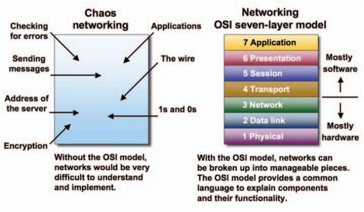
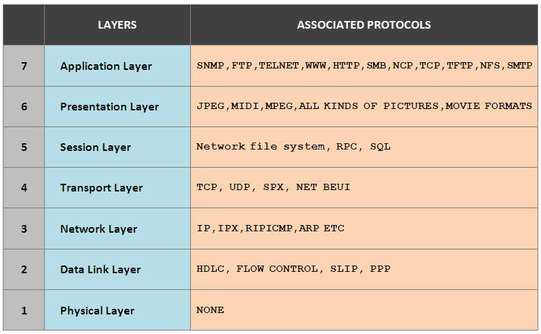
OSI Model

The Open System Interconnection (OSI) model is a reference tool for understanding data communication between any two networked systems. It divides the communication processes into 7 layers. Each layer performs specific functions to support the layers above it and uses services of the layers below it.

Physical Layer: The physical layer coordinates the functions required to transmit a bit stream over a physical medium. It deals with the mechanical and electrical specifications of interface and transmission medium. It also defines the procedures and functions that physical devices and interfaces have to perform for transmission to occur.

Data Link Layer: The data link layer transforms the physical layer, a raw transmission facility, to a reliable link and is responsible for Node-to-Node delivery. It makes the physical layer appear error free to the upper layer (i.e, network layer).

Network Layer: Network layer is responsible for source to destination delivery of a packet possibly across multiple networks (links). If the two systems are connected to the same link, there is usually no need for a network layer. However, if the two systems are attached to different networks (links) with connecting devices between networks, there is often a need of the network layer to accomplish source to destination delivery.

Transport Layer: The transport layer is responsible for- source to destination (end-to-end) delivery of the entire message. Network layer does not recognise any relationship between the packets delivered. Network layer treats each packet independently, as though each packet belonged to a separate message, whether or not it does. The transport layer ensures that the whole message arrives intact and in order.

Session Layer: The session layer is the network dialog controller. It establishes, maintains and synchronises the interaction between communicating systems. It also plays important role in keeping applications data separate.

Presentation Layer: This layer is responsible for how an application formats data to be sent out onto the network. This layer basically allows an application to read (or understand) the message.

Ethernet
It is basically a LAN technology which strikes a good balance between speed, cost and ease of installation.

• Ethernet topologies are generally bus and/or bus-star topologies.
• Ethernet networks are passive, which means Ethernet hubs do not reprocess or alter the signal sent by the attached devices.
• Ethernet technology uses broadcast topology with baseband signalling and a control method called Carrier Sense Multiple Access/Collision Detection (CSMA/CD) to transmit data.
• The IEEE 802.3 standard defines Ethernet protocols for (Open Systems Interconnect) OSI’s Media Access Control (MAC) sublayer and physical layer network characteristics.
• The IEEE 802.2 standard defines protocols for the Logical Link Control (LLC) sublayer.

 Ethernet refers to the family of local area network (LAN) implementations that include three principal categories.

• Ethernet and IEEE 802.3: LAN specifications that operate at 10 Mbps over coaxial cable.
• 100-Mbps Ethernet: A single LAN specification, also known as Fast Ethernet, which operates at 100 Mbps over twisted-pair cable.
• 1000-Mbps Ethernet: A single LAN specification, also known as Gigabit Ethernet, that operates at 1000 Mbps (1 Gbps) over fiber and twisted-pair cables.

IEEE Standards

• IEEE 802.1: Standards related to network management.
• IEEE 802.2: Standard for the data link layer in the OSI Reference Model
• IEEE 802.3: Standard for the MAC layer for bus networks that use CSMA/CD. (Ethernet standard)
• IEEE 802.4: Standard for the MAC layer for bus networks that use a token-passing mechanism (token bus networks).
• IEEE 802.5: Standard for the MAC layer for token-ring networks.
• IEEE 802.6: Standard for Metropolitan Area Networks (MANs).
• 

FLOW CONTROL:

Flow control coordinates that amount of data that can be sent before receiving ACK It is one of the most important duties of the data link layer.

ERROR CONTROL: Error control in the data link layer is based on ARQ (automatic repeat request), which is the retransmission of data.

• The term error control refers to methods of error detection and retransmission.
• Anytime an error is detected in an exchange, specified frames are retransmitted. This process is called ARQ.

Error Control (Detection and Correction)

Many factors including line noise can alter or wipe out one or more bits of a given data unit.

 

• Reliable systems must have mechanism for detecting and correcting such errors.
• Error detection and correction are implemented either at the data link layer or the transport layer of the OSI model.

 Error Detection

Error detection uses the concept of redundancy, which means adding extra bits for detecting errors at the destination.

Note: Checking function performs the action that the received bit stream passes the checking criteria, the data portion of the data unit is accepted else rejected.

Vertical Redundancy Check (VRC)

In this technique, a redundant bit, called parity bit, is appended to every data unit, so that the total number of 1’s in the unit (including the parity bit) becomes even. If number of 1’s are already even in data, then parity bit will be 0.

Some systems may use odd parity checking, where the number of 1’s should be odd. The principle is the same, the calculation is different.

 Checksum

There are two algorithms involved in this process, checksum generator at sender end and checksum checker at receiver end.

The sender follows these steps

• The data unit is divided into k sections each of n bits.
• All sections are added together using 1’s complement to get the sum.
• The sum is complemented and becomes the checksum.
• The checksum is sent with the data.

 The receiver follows these steps

• The received unit is divided into k sections each of n bits.
• All sections are added together using 1’s complement to get the sum.
• The sum is complemented.
• If the result is zero, the data are accepted, otherwise they are rejected.

Cyclic Redundancy Check (CRC): CRC is based on binary division. A sequence of redundant bits called CRC or the CRC remainder is appended to the end of a data unit, so that the resulting data unit becomes exactly divisible by a second, predetermined binary number. At its destination, the incoming data unit is divided by the same number. If at this step there is no remainder, the data unit is assumed to be intact and therefore is accepted.

Error Correction: Error correction in data link layer is implemented simply anytime, an error is detected in an exchange, a negative acknowledgement NAK is returned and the specified frames are retransmitted. This process is called Automatic Repeat Request (ARQ). Retransmission of data happens in three Cases: Damaged frame, Lost frame and Lost acknowledgement.

 Stop and Wait ARQ: Include retransmission of data in case of lost or damaged framer. For retransmission to work, four features are added to the basic flow control mechanism.

• If an error is discovered in a data frame, indicating that it has been corrupted in transit, a NAK frame is returned. NAK frames, which are numbered, tell the sender to retransmit the last frame sent.
• The sender device is equipped with a timer. If an expected acknowledgement is not received within an allotted time period, the sender assumes that the last data frame was lost in transmit and sends it again.

 Sliding Window ARQ: To cover retransmission of lost or damaged frames, three features are added to the basic flow control mechanism of sliding window.

• The sending device keeps copies of all transmitted frames, until they have been acknowledged. .
• In addition to ACK frames, the receiver has the option of returning a NAK frame, if the data have been received damaged. NAK frame tells the sender to retransmit a damaged frame. Here, both ACK and NAK frames must be numbered for identification. ACK frames carry the number of next frame expected. NAK frames on the other hand, carry the number of the damaged frame itself. If the last ACK was numbered 3, an ACK 6 acknowledges the receipt of frames 3, 4 and 5 as well. If data frames 4 and 5 are received damaged, both NAK 4 and NAK 5 must be returned.
• Like stop and wait ARQ, the sending device in sliding window ARQ is equipped with a timer to enable it to handle lost acknowledgements.

 Go-back-n ARQ: In this method, if one frame is lost or damaged all frames sent, since the last frame acknowledged are retransmitted.

Selective Reject ARQ: In this method, only specific damaged or lost frame is retransmitted. If a frame is corrupted in transmit, a NAK is returned and the frame is resent out of sequence. The receiving device must be able to sort the frames it has and insert the retransmitted frame into its proper place in the sequence.

 Flow Control

One important aspect of data link layer is flow control. Flow control refers to a set of procedures used to restrict the amount of data the sender can send before waiting for acknowledgement.

Stop and Wait: In this method, the sender waits for an acknowledgement after every frame it sends. Only when a acknowledgment has been received is the next frame sent. This process continues until the sender transmits an End of Transmission (EOT) frame.

• We can have two ways to manage data transmission, when a fast sender wants to transmit data to a low speed receiver.
• The receiver sends information back to sender giving it permission to send more data i.e., feedback or acknowledgment based flow control.
• Limit the rate at which senders may transmit data without using feedback from receiver i.e., Rate based-flow control.

Advantages of Stop and Wait:

It’s simple and each frame is checked and acknowledged well.

Disadvantages of Stop and Wait:

• It is inefficient, if the distance between devices is long.
• The time spent for waiting ACKs between each frame can add significant amount to the total transmission time.

Sliding Window: In this method, the sender can transmit several frames before needing an acknowledgement. The sliding window refers imaginary boxes at both the sender and the receiver. This window can hold frames at either end and provides the upper limit on the number of frames that can be transmitted before requiring an acknowledgement.

• The frames in the window are numbered modulo-n, which means they are numbered from 0 to n -1. For example, if n = 8, the frames are numbered 0, 1, 2, 3, 4, 5, 6, 7, 0, 1, 2, 3, 4, 5, 6, 7, 0, 1…so on. The size of the window is (n -1) in this case size of window = 7. .
• In other words, the window can’t cover the whole module (8 frames) it covers one frame less that is 7.
• When the receiver sends an ACK, it includes the number of the next frame it expects to receive. When the receiver sends an ACK containing the number 5, it means all frames upto number 4 have been received.

Switching

Whenever, we have multiple devices we have a problem of how to connect them to make one-to-one communication possible. Two solutions could be like as given below

• Install a point-to-point connection between each pair of devices (Impractical and wasteful approach when applied to very large network).
• For large network, we can go for switching. A switched network consists of a series of interlinked nodes, called switches.

 

Classification of Switching

Circuit Switching: It creates a direct physical connection between two devices such as phones or computers.

Space Division Switching: Separates the path in the circuit from each other spatially.

Time Division Switching: Uses time division multiplexing to achieve switching. Circuit switching was designed for voice communication. In a telephone conversation e.g., Once a circuit is established, it remains connected for the duration of the session.

 Disadvantages of Circuit Switching

• Less suited to data and other non-voice transmissions.
• A circuit switched link creates the equivalent of a single cable between two devices and thereby assumes a single data rate for both devices. This assumption limits the flexibility and usefulness of a circuit switched connection.
• Once a circuit has been established, that circuit is the path taken by all parts of the transmission, whether or not it remains the most efficient or available.
• Circuit switching sees all transmissions as equal. Any request is granted to whatever link is available. But often with data transmission, we want to be able to prioritise.

 Packet Switching

To overcome the disadvantages of circuit switch. Packet switching concept came into the picture.

In a packet switched network, data are transmitted in discrete units of potentially variable length blocks called packets. Each packet contains not only data but also a header with control information (such as priority codes and source and destination address). The packets are sent over the network node to node. At each node, the packet is stored briefly, then routed according to the information in its header.

There are two popular approaches to packet switching.

1. Datagram
2. Virtual circuit

Datagram Approach: Each packet is treated independently from all others. Even when one packet represents just a piece of a multi packet transmission, the network (and network layer functions) treats it as though it existed alone.

Virtual Circuit Approach: The relationship between all packets belonging to a message or session is preserved. A single route is chosen between sender and receiver at the beginning of the session. When the data are sent, all packets of the transmission travel one after another along that route.

We can implement it into two formats:

• Switched Virtual Circuit (SVC)
• Permanent Virtual Circuit (PVC)

SVC (Switched Virtual Circuit)

This SVC format is comparable conceptually to dial-up lines in circuit switching. In this method, a virtual circuit is created whenever, it is needed and exists only for the duration of the specific exchange.

PVC (Permanent Virtual Circuit)

The PVC format is comparable to leased lines in circuit switching. In this method, the same virtual circuit is provided between two users on a continuous basis. The circuit is dedicated to the specific users. No one else can use it and because it is always in place, it can be used without connection establishment and connection termination.

Message Switching

It is also known as store and forward. In this mechanism, a node receives a message, stores it, until the appropriate route is free, and then sends it along.

Store and forward is considered a switching technique because there is no direct link between the sender and receiver of a transmission. A message is delivered to the node along one path, then rerouted along another to its destination.

In message switching, the massages are stored and relayed from secondary storage (disk), while in packet switching the packets are stored and forwarded from primary storage (RAM).

Internet Protocol: It is a set of technical rules that defines how computers communicate over a network.

IPv4: It is the first version of Internet Protocol to be widely used, and accounts for most of today’s Internet traffic.

• Address Size: 32 bits
• Address Format: Dotted Decimal Notation: 192.149.252.76
• Number of Addresses: 2³² = 4,294,967,296 Approximately
• IPv4 header has 20 bytes
• IPv4 header has many fields (13 fields)
• It is subdivided into classes <A-E>.
• Address uses a subnet mask.
• IPv4 has lack of security.

 

 

IPv6: It is a newer numbering system that provides a much larger address pool than IPv4.

• Address Size: 128 bits
• Address Format: Hexadecimal Notation: 3FFE:F200:0234:AB00: 0123:4567:8901:ABCD
• Number of Addresses: 2¹²⁸
• IPv6 header is the double, it has 40 bytes
• IPv6 header has fewer fields, it has 8 fields.
• It is classless.
• It uses a prefix and an Identifier ID known as IPv4 network
• It uses a prefix length.
• It has a built-in strong security (Encryption and Authentication)

 Classes and Subnetting

There are currently five different field length pattern in use, each defining a class of address.

An IP address is 32 bit long. One portion of the address indicates a network (Net ID) and the other portion indicates the host (or router) on the network (i.e., Host ID).

To reach a host on the Internet, we must first reach the network, using the first portion of the address (Net ID). Then, we must reach the host itself, using the 2nd portion (Host ID).

The further division a network into smaller networks called subnetworks.

For Class A: First bit of Net ID should be 0 like in following pattern

01111011 . 10001111 . 1111100 . 11001111

 

For Class B: First 2 bits of Net ID should be 1 and 0 respective, as in below

pattern 10011101 . 10001111 . 11111100 . 11001111

 

For Class C: First 3 bits Net ID should be 1, 1 and 0 respectively, as follows

11011101 . 10001111 . 11111100 . 11001111

 

For Class D: First 4 bits should be 1110 respectively, as in pattern

11101011 . 10001111 . 11111100 . 11001111

 

For Class E: First 4 bits should be 1111 respectively, like

11110101 . 10001111 . 11111100 . 11001111

 

Class Ranges of Internet Address in Dotted Decimal Format

Three Levels of Hierarchy: Adding subnetworks creates an intermediate level of hierarchy in the IP addressing system. Now, we have three levels: net ID; subnet ID and host ID. e.g.,

 Masking

Masking is process that extracts the address of the physical network form an IP address. Masking can be done whether we have subnetting or not. If we have not subnetted the network, masking extracts the network address form an IP address. If we have subnetted, masking extracts the subnetwork address form an IP address. 

 

Masks without Subnetting: To be compatible, routers use mask even, if there is no subneting.

 

Masks with Subnetting: When there is subnetting, the masks can vary

Masks for Unsubnetted Networks

Masks for Subnetted Networks

 

Types of Masking

There are two types of masking as given below

 

Boundary Level Masking: If the masking is at the boundary level (the mask numbers are either 255 or 0), finding the subnetwork address is very easy. Follow these 2 rules

• The bytes in IP address that correspond to 255 in the mask will be repeated in the subnetwork address.
• The bytes in IP address that correspond to 0 in the mask will change to 0 in the subnetwork address.

 

Non-boundary Level Masking: If the masking is not at the boundary level (the mask numbers are not just 255 or 0), finding subnetwork address involves using the bit-wise AND operator, follow these 3 rules

• The bytes in IP address that correspond to 255 in the mask will be repeated in the subnetwork address.
• The bytes in the IP address that correspond to 0 in the mask will be change to 0 in the subnetwork address.
• For other bytes, use the bit-wise AND operator
• 

As we can see, 3 bytes are ease {, to determine. However, the 4th bytes needs the bit-wise AND operation.

Router: A router is a hardware component used to interconnect networks. Routers are devices whose primary purpose is to connect two or more networks and to filter network signals so that only desired information travels between them. Routers are much more powerful than bridges.

• A router has interfaces on multiple networks
• Networks can use different technologies
• Router forwards packets between networks
• Transforms packets as necessary to meet standards for each network
• Routers are distinguished by the functions they perform:
  • Internal routers: Only route packets within one area.
  • Area border routers: Connect to areas together
  • Backbone routers: Reside only in the backbone area
  • AS boundary routers: Routers that connect to a router outside the AS.

Routers can filter traffic so that only authorized personnel can enter restricted areas. They can permit or deny network communications with a particular Web site. They can recommend the best route for information to travel. As network traffic changes during the day, routers can redirect information to take less congested routes.

• Routers operate primarily by examining incoming data for its network routing and transport information.
• Based on complex, internal tables of network information that it compiles, a router then determines whether or not it knows how to forward the data packet towards its destination.
• Routers can be programmed to prevent information from being sent to or received from certain networks or computers based on all or part of their network routing addresses.
• Routers also determine some possible routes to the destination network and then choose the one that promises to be the fastest.

 

Two key router functions of Router:

• Run routing algorithms/protocol (RIP, OSPF, BGP)
• Forwarding datagrams from incoming to outgoing link.

Address Resolution Protocol (ARP)

ARP is used to find the physical address of the node when its Internet address is known. Anytime, a host or a router needs to find the physical address of another has on its network; it formats an ARP query packet that includes that IP address and broadcasts it over the network. Every host on the network receives and processes the ARP packet, but the intended recipient recognises its Internet address and sends back its physical address.

Reverse Address Resolution Protocol (RARP)

This protocol allows a host to discover its Internet address when it known only its physical address. RARP works much like ARP. The host wishing to retrieve its Internet address broadcasts an RARP query packet that contains its physical address to every host of its physical network. A server on the network recognises the RARP packet and return the hosts Internet address.

Internet Control Massage Protocol (ICMP)

The ICMP is a mechanism used by hosts and routers to send notifications of datagram problems back to the sender. IP is essentially an unreliable and connectionless protocol. ICMP allows IP (Internet Protocol) to inform a sender, if a datagram is undeliverable.

ICMP uses each test/reply to test whether a destination is reachable and responding. It also handles both control and error massages but its sole function is to report problems not correct them.

Internet Group Massage Protocol (IGMP)

The IP can be involved in two types of communication unitasking and multitasking. The IGMP protocol has been designed to help a multitasking router to identify the hosts in a LAN that are members of a multicast group.

Addressing at Network Layer

In addition to the physical addresses that identify individual devices, the Internet requires an additional addressing connection an address that identifies the connection of a host of its network. Every host and router on the Internet has an IP address which encodes its network number and host number. The combination is unique in principle; no 2 machines on the Internet have the same IP address.

Firewall

A firewall is a device that prevents unauthorized electronic access to your entire network.

The term firewall is generic, and includes many different kinds of protective hardware and software devices. Routers, comprise one kind of firewall.

Most firewalls operate by examining incoming or outgoing packets for information at OSI level 3, the network addressing level.

Firewalls can be divided into 3 general categories: packet-screening firewalls, proxy servers (or application-level gateways), and stateful inspection proxies.

• Packet-screening firewalls examine incoming and outgoing packets for their network address information. You can use packet-screening firewalls to restrict access to specific Web sites, or to permit access to your network only from specific Internet sites.
• Proxy servers (also called application-level gateways) operate by examining incoming or outgoing packets not only for their source or destination addresses but also for information carried within the data area (as opposed to the address area) of each network packet. The data area contains information written by the application program that created the packet—for example, your Web browser, FTP, or TELNET program. Because the proxy server knows how to examine this application-specific portion of the packet, you can permit or restrict the behavior of individual programs.
• Stateful inspection proxies monitor network signals to ensure that they are part of a legitimate ongoing conversation (rather than malicious insertions)

Transport Layer Protocols: There are two transport layer protocols as given below.

UDP (User Datagram Protocol)

UDP is a connection less protocol. UDP provides a way for application to send encapsulate IP datagram and send them without having to establish a connection.

• Datagram oriented
• unreliable, connectionless
• simple
• unicast and multicast
• Useful only for few applications, e.g., multimedia applications
• Used a lot for services: Network management (SNMP), routing (RIP), naming (DNS), etc.

UDP transmitted segments consisting of an 8 byte header followed by the payload. The two parts serve to identify the end points within the source and destinations machine. When UDP packets arrives, its payload is handed to the process attached to the destination ports.

• Source Port Address (16 Bits)

Total length of the User Datagram (16 Bits)

• Destination Port Address (16 Bits)

Checksum (used for error detection) (16 Bits

TCP (Transmission Control Protocol)

TCP provides full transport layer services to applications. TCP is reliable stream transport port-to-port protocol. The term stream in this context, means connection-oriented, a connection must be established between both ends of transmission before either may transmit data. By creating this connection, TCP generates a virtual circuit between sender and receiver that is active for the duration of transmission.

TCP is a reliable, point-to-point, connection-oriented, full-duplex protocol.

Flag bits

• URG: Urgent pointer is valid If the bit is set, the following bytes contain an urgent message in the sequence number range “SeqNo <= urgent message <= SeqNo + urgent pointer”
• ACK: Segment carries a valid acknowledgement
• PSH: PUSH Flag, Notification from sender to the receiver that the receiver should pass all data that it has to the application. Normally set by sender when the sender’s buffer is empty
• RST: Reset the connection, The flag causes the receiver to reset the connection. Receiver of a RST terminates the connection and indicates higher layer application about the reset
• SYN: Synchronize sequence numbers, Sent in the first packet when initiating a connection
• FIN: Sender is finished with sending. Used for closing a connection, and both sides of a connection must send a FIN.

TCP segment format

Each machine supporting TCP has a TCP transport entity either a library procedure, a user process or port of kernel. In all cases, it manages TCP streams and interfaces to the IP layer. A TCP entities accepts the user data stream from local processes, breaks them up into pieces not exceeding 64 K bytes and sends each piece as separate IP datagrams.

Sockets

A socket is one end of an inter-process communication channel. The two processes each establish their own socket. The system calls for establishing a connection are somewhat different for the client and the server, but both involve the basic construct of a socket.

The steps involved in establishing a socket on the client side are as follows:

1. Create a socket with the socket() system call
2. Connect the socket to the address of the server using the connect() system call
3. Send and receive data. There are a number of ways to do this, but the simplest is to use the read() and write() system calls.

The steps involved in establishing a socket on the server side are as follows:

1. Create a socket with the socket() system call
2. Bind the socket to an address using the bind() system call. For a server socket on the Internet, an address consists of a port number on the host machine.
3. Listen for connections with the listen() system call
4. Accept a connection with the accept() system call. This call typically blocks until a client connects with the server.
5. Send and receive data

When a socket is created, the program has to specify the address domain and the socket type.

 

Socket Types

There are two widely used socket types, stream sockets, and datagram sockets.

Stream sockets treat communications as a continuous stream of characters, while datagram sockets have to read entire messages at once. Each uses its own communications protocol. Stream sockets use TCP (Transmission Control Protocol), which is a reliable, stream oriented protocol, and datagram sockets use UDP (Unix Datagram Protocol), which is unreliable and message oriented. A second type of connection is a datagram socket. You might want to use a datagram socket in cases where there is only one message being sent from the client to the server, and only one message being sent back. There are several differences between a datagram socket and a stream socket.

1. Datagrams are unreliable, which means that if a packet of information gets lost somewhere in the Internet, the sender is not told (and of course the receiver does not know about the existence of the message). In contrast, with a stream socket, the underlying TCP protocol will detect that a message was lost because it was not acknowledged, and it will be retransmitted without the process at either end knowing about this.
2. Message boundaries are preserved in datagram sockets. If the sender sends a datagram of 100 bytes, the receiver must read all 100 bytes at once. This can be contrasted with a stream socket, where if the sender wrote a 100 byte message, the receiver could read it in two chunks of 50 bytes or 100 chunks of one byte.
3. The communication is done using special system calls sendto() and receivefrom() rather than the more generic read() and write().
4. There is a lot less overhead associated with a datagram socket because connections do not need to be established and broken down, and packets do not need to be acknowledged. This is why datagram sockets are often used when the service to be provided is short, such as a time-of-day service.

Application Layer Protocols (DNS, SMTP, POP, FTP, HTTP)

There are various application layer protocols as given below

• SMTP (Simple Mail Transfer Protocol): One of the most popular network service is electronic mail (e-mail). The TCP/IP protocol that supports electronic mail on the Internet is called Simple Mail Transfer Protocol (SMTP). SMTP is system for sending messages to other computer. Users based on e-mail addresses. SMTP provides services for mail exchange between users on the same or different computers.
• TELNET (Terminal Network): TELNET is client-server application that allows a user to log onto remote machine and lets the user to access any application program on a remote computer. TELNET uses the NVT (Network Virtual Terminal) system to encode characters on the local system. On the server (remote) machine, NVT decodes the characters to a form acceptable to the remote machine.
• FTP (File Transfer Protocol): FTP is the standard mechanism provided by TCP/IP for copying a file from one host to another. FTP differs form other client-server applications because it establishes 2 connections between hosts. One connection is used for data transfer, the other for control information (commands and responses).
• Multipurpose Internet Mail Extensions (MIME): It is an extension of SMTP that allows the transfer of multimedia messages.
• POP (Post Office Protocol): This is a protocol used by a mail server in conjunction with SMTP to receive and holds mail for hosts.
• HTTP (Hypertext Transfer Protocol): This is a protocol used mainly to access data on the World Wide Web (www), a respository of information spread all over the world and linked together. The HTIP protocol transfer data in the form of plain text, hyper text, audio, video and so on.
• Domain Name System (DNS): To identify an entity, TCP/IP protocol uses the IP address which uniquely identifies the connection of a host to the Internet. However, people refer to use names instead of address. Therefore, we need a system that can map a name to an address and conversely an address to name. In TCP/IP, this is the domain name system.

DNS in the Internet

DNS is protocol that can be used in different platforms. Domain name space is divided into three categories.

• Generic Domain: The generic domain defines registered hosts according, to their generic behaviour. Each node in the tree defines a domain which is an index to the domain name space database.

• Country Domain: The country domain section follows the same format as the generic domain but uses 2 characters country abbreviations (e.g., US for United States) in place of 3 characters.
• Inverse Domain: The inverse domain is used to map an address to a name.

 

Overview of Services

 

Network Security: As millions of ordinary citizens are using networks for banking, shopping, and filling their tax returns, network security is looming on the horizon as a potentially massive problem.

 Network security problems can be divided roughly into four interwined areas:

1. Secrecy: keep information out of the hands of unauthorized users.
2. Authentication: deal with determining whom you are talking to before revealing sensitive information or entering into a business deal.
3. Nonrepudiation: deal with signatures.
4. Integrity control: how can you be sure that a message you received was really the one sent and not something that a malicious adversary modified in transit or concocted?

There is no one single place — every layer has something to contribute:

• In the physical layer, wiretapping can be foiled by enclosing transmission lines in sealed tubes containing argon gas at high pressure. Any attempt to drill into a tube will release some gas, reducing the pressure and triggering an alarm (used in some military systems).
• In the data link layer, packets on a point-to-point line can be encoded.
• In the network layer, firewalls can be installed to keep packets in/out.
• In the transport layer, entire connection can be encrypted.

Model for Network Security

Network security starts with authenticating, commonly with a username and password since, this requires just one detail authenticating the username i.e., the password this is some times teamed one factor authentication.

Using this model require us to

• Design a suitable algorithm for the security transformation.
• Generate the secret in formations (keys) used by the algorithm.
• Develop methods to distribute and share the secret information.
• Specify a protocol enabling the principles to use the transformation and secret information for security service.

Cryptography

It is a science of converting a stream of text into coded form in such a way that only the sender and receiver of the coded text can decode the text. Nowadays, computer use requires automated tools to protect files and other stored information. Uses of network and communication links require measures to protect data during transmission.

Symmetric / Private Key Cryptography (Conventional / Private key / Single key)

Symmetric key algorithms are a class of algorithms to cryptography that use the same cryptographic key for both encryption of plaintext and decryption of ciphertext. The may be identical or there may be a simple transformation to go between the two keys.

In symmetic private key cryptography the following key features are involved

• Sender and recipient share a common key.
• It was only prior to invention of public key in 1970.
• If this shared key is disclosed to opponent, communications are compromised.
• Hence, does not protect sender form receiver forging a message and claiming is sent by user.

Advantage of Secret key Algorithm: Secret Key algorithms are efficient: it takes less time to encrypt a message. The reason is that the key is usually smaller. So it is used to encrypt or decrypt long messages.

 Disadvantages of Secret key Algorithm: Each pair of users must have a secret key. If N people in world want to use this method, there needs to be N (N-1)/2 secret keys. For one million people to communicate, a half-billion secret keys are needed. The distribution of the keys between two parties can be difficult.

Asymmetric / Public Key Cryptography

A public key cryptography refers to a cyptogaphic system requiring two separate keys, one of which is secrete/private and one of which is public although different, the two pats of the key pair are mathematically linked.

• Public Key: A public key, which may be known by anybody and can be used to encrypt messages and verify signatures.
• Private Key: A private key, known only to the recipient, used to decrypt messages and sign (create) signatures. It is symmetric because those who encrypt messages or verify signature cannot decrypt messages or create signatures. It is computationally infeasible to find decryption key knowing only algorithm and encryption key. Either of the two related keys can be used for encryption, with the other used for decryption (in some schemes).

 

In the above public key cryptography mode

• Bob encrypts a plaintext message using Alice’s public key using encryption algorithm and sends it over communication channel.
• On the receiving end side, only Alice can decrypt this text as she only is having Alice’s private key.

Advantages of Public key Algorithm:

1. Remove the restriction of a shared secret key between two entities. Here each entity can create a pair of keys, keep the private one, and publicly distribute the other one.
2. The no. of keys needed is reduced tremendously. For one million users to communicate, only two million keys are needed.

Disadvantage of Public key Algorithm: If you use large numbers the method to be effective. Calculating the cipher text using the long keys takes a lot of time. So it is not recommended for large amounts of text.

Message Authentication Codes (MAC)

In cryptography, a Message Authentication Code (MAC) is a short piece of information used to authenticate a message and to provide integrity and authenticity assurance on the message. Integrity assurance detects accidental and international message changes, while authenticity assurance affirms the message’s origin.

A keyed function of a message sender of a message m computers MAC (m) and appends it to the message.

Verification: The receiver also computers MAC (m) and compares it to the received value.

Security of MAC: An attacker should not be able to generate a valid (m, MAC (m)), even after seeing many valid messages MAC pairs, possible of his choice.

MAC from a Block Cipher

MAC from a block cipher can be obtained by using the following suggestions

• Divide a massage into blocks.
• Compute a checksum by adding (or xoring) them.
• Encrypt the checksum.
• MAC keys are symmetric. Hence, does not provide non-repudiation (unlike digital signatures).
• MAC function does not need to be invertiable.
• A MACed message is not necessarily encrypted.

 

 

DES (Data Encryption Standard)

• The data encryption standard was developed in IBM.
• DES is a symmetric key crypto system.
• It has a 56 bit key.
• It is block cipher, encrypts 64 bit plain text to 64 bit cipher texts.
• Symmetric cipher: uses same key for encryption and decryption
• It Uses 16 rounds which all perform the identical operation.
• Different subkey in each round derived from main key
• Depends on 4 functions: Expansion E, XOR with round key, S-box substitution, and Permutation.
• DES results in a permutation among the 2⁶⁴ possible arrangements of 64 bits, each of which may be either 0 or 1. Each block of 64 bits is divided into two blocks of 32 bits each, a left half block L and a right half R. (This division is only used in certain operations.)

DES is a block cipher–meaning it operates on plaintext blocks of a given size (64-bits) and returns cipher text blocks of the same size. Thus DES results in a permutation among the 2⁶⁴possible arrangements of 64 bits, each of which may be either 0 or 1. Each block of 64 bits is divided into two blocks of 32 bits each, a left half block L and a right half R. (This division is only used in certain operations.)

Authentication Protocols

Authentication: It is the technique by which a process verifies that its communication partner is who it is supposed to be and not an imposter. Verifying the identity of a remote process in the face of a malicious, active intruder is surprisingly difficult and requires complex protocols based on cryptography.

 The general model that all authentication protocols use is the following:

• An initiating user A (for Alice) wants to establish a secure connection with a second user B (for Bob). Both and are sometimes called principals.
• Starts out by sending a message either to, or to a trusted key distribution center (KDC), which is always honest. Several other message exchanges follow in various directions.
• As these message are being sent, a nasty intruder, T (for Trudy), may intercept, modify, or replay them in order to trick and When the protocol has been completed, is sure she is talking to and is sure he is talking to. Furthermore, in most cases, the two of them will also have established a secret session key for use in the upcoming conversation.

In practice, for performance reasons, all data traffic is encrypted using secret-key cryptography, although public-key cryptography is widely used for the authentication protocols themselves and for establishing the (secret) session key.

Authentication based on a shared Secret key

Assumption: and share a secret key, agreed upon in person or by phone.

This protocol is based on a principle found in many (challenge-response) authentication protocols: one party sends a random number to the other, who then transforms it in a special way and then returns the result.

 Three general rules that often help are as follows:

1. Have the initiator prove who she is before the responder has to.
2. Have the initiator and responder use different keys for proof, even if this means having two shared keys, and.
3. Have the initiator and responder draw their challenges from different sets.

Authentication using Public-key Cryptography

Assume that and already know each other’s public keys (a nontrivial issue).

 Digital Signatures: For computerized message systems to replace the physical transport of paper and documents, a way must be found to send a “signed” message in such a way that

1. The receiver can verify the claimed identity of the sender.
2. The sender cannot later repudiate the message.
3. The receiver cannot possibly have concocted the message himself.

 Secret-key Signatures: Assume there is a central authority, Big Brother (BB), that knows everything and whom everyone trusts.

 If later denies sending the message, how could prove that indeed sent the message?

• First points out that will not accept a message from unless it is encrypted with.
• Then produces, and says this is a message signed by which proves sent to.
• is asked to decrypt , and testifies that is telling the truth.

What happens if replays either message?

• can check all recent messages to see if was used in any of them (in the past hour).
• The timestamp is used throughout, so that very old messages will be rejected based on the timestamp.

Public-key Signatures: It would be nice if signing documents did not require a trusted authority (e.g., governments, banks, or lawyers, which do not inspire total confidence in all citizens).

Under this condition,

• sends a signed message to by transmitting .
• When receives the message, he applies his secret key to get , and saves it in a safe place, then applies the public key to get .
• How to verify that indeed sent a message to ?
• Produces both and The judge can easily verify that indeed has a valid message encrypted by simply applying to it. Since is private, the only way could have acquired a message encrypted by it is if did indeed send it.

Another new standard is the Digital Signature Standard (DSS) based on the EI Gamal public-key algorithm, which gets its security from the difficulty of computing discrete logarithms, rather than factoring large numbers.

Message Digest

• It is easy to compute.
• No one can generate two messages that have the same message digest.
• To sign a plaintext, first computes, and performs , and then sends both and to .
• When everything arrives, applies the public key to the signature part to yield, and applies the well-known to see if the so computed agrees with what was received (in order to reject the forged message).

Data Structure

A data structure is a specialised way for organising and storing data in memory, so that one can perform operations on it.

For example:

We have data player’s name “Dhoni” and age 35. Here “Dhoni” is of String data type and 35 is of integer data type.

Now we can organise this data as a record like Player record.

We can collect and store player’s records in a file or database as a data structure.

For example: “Dhoni” 35, “Rahul” 24, “Rahane” 28.

“Data Structures are structures programmed to store ordered data so that various operations can be performed on it easily.”

Data structure is all about:

• How to represent data element(s).
• What relationship data elements have among themselves.
• How to access data elements i.e., access methods

Types of Data Structure:

Primitive Data Structures : Integer, Float, Boolean, Char etc, all are data structures.

Abstract Data Structure: Used to store large and connected data.

• Linked List
• Tree
• Graph
• Stack, Queue etc.

Operations on Data Structures: The operations involve in data structure are as follows.

• Create: Used to allocate/reserve memory for the data element(s).
• Destroy: This operation deallocate/destroy the memory space assigned to the specified data structure.
• Selection: Accessing a particular data within a data structure.
• Update: For updation (insertion or deletion) of data in the data structure.
• Searching: Used to find out the presence of the specified data item in the list of data item.
• Sorting: Process of arranging all data items either in ascending or in descending order.
• Merging: Process of combining data items of two different sorted lists of data items into a single list.

Stack

A stack is an ordered collection of items into which new items may be inserted and from which items may be deleted at one end, called the TOP of the stack. It is a LIFO (Last In First Out) kind of data structure.

Operations on Stack:

• Push: Adds an item onto the stack. PUSH (s, i); Adds the item i to the top of stack.
• Pop: Removes the most-recently-pushed item from the stack. POP (s); Removes the top element and returns it as a function value.
• size(): It returns the number of elements in the queue.
• isEmpty(): It returns true if queue is empty.

Implementation of Stack: A stack can be implemented using two ways: Array and Linked list.

But since array sized is defined at compile time, it can’t grow dynamically. Therefore, an attempt to insert/push an element into stack (which is implemented through array) can cause a stack overflow situation, if it is already full.

Go, to avoid the above mentioned problem we need to use linked list to implement a stack, because linked list can grow dynamically and shrink at runtime.

Applications of Stack: There are many applications of stack some of the important applications are given below.

• Backtracking. This is a process when you need to access the most recent data element in a series of elements.
• Depth first Search can be implemented.
• Function Calls: Different ways of organising the data are known as data structures.
• Simulation of Recursive calls: The compiler uses one such data structure called stack for implementing normal as well as recursive function calls.
• Parsing: Syntax analysis of compiler uses stack in parsing the program.
• Expression Evaluation: How a stack can be used for checking on syntax of an expression.
  • Infix expression: It is the one, where the binary operator comes between the operands.
    e. g., A + B * C.
  • Postfix expression: Here, the binary operator comes after the operands.
    e.g., ABC * +
  • Prefix expression: Here, the binary operator proceeds the operands.
    e.g.,+ A * BC

This prefix expression is equivalent to A + (B * C) infix expression. Prefix notation is also known as Polish notation. Postfix notation is also known as suffix or Reverse Polish notation.

• Reversing a List: First push all the elements of string in stack and then pop elements.
• Expression conversion: Infix to Postfix, Infix to Prefix, Postfix to Infix, and Prefix to Infix
• Implementation of Towers of Hanoi
• Computation of a cycle in the graph

Queue

It is a non-primitive, linear data structure in which elements are added/inserted at one end (called the REAR) and elements are removed/deleted from the other end (called the FRONT). A queue is logically a FIFO (First in First Out) type of list.

Operations on Queue:

• Enqueue: Adds an item onto the end of the queue ENQUEUE(Q, i); Adds the item i onto the end of queue.
• Dequeue: Removes the item from the front of the queue. DEQUEUE (Q); Removes the first element and returns it as a function value.

Queue Implementation: Queue can be implemented in two ways.

• Static implementation (using arrays)
• Dynamic implementation (using painters)

Circular Queue: In a circular queue, the first element comes just after the last element or a circular queue is one in which the insertion of a new element is done at the very first location of the queue, if the last location of queue is full and the first location is empty.

Note:- A circular queue overcomes the problem of unutilised space in linear queues implemented as arrays.

We can make following assumptions for circular queue.

• Front will always be pointing to the first element (as in linear queue).
• If Front = Rear, the queue will be empty.
• Each time a new element is inserted into the queue, the Rear is incremented by 1.
  Rear = Rear + 1
• Each time, an element is deleted from the queue, the value of Front is incremented by one.
  Front = Front + 1

Double Ended Queue (DEQUE): It is a list of elements in which insertion and deletion operations are performed from both the ends. That is why it is called double-ended queue or DEQUE.

Priority Queues: This type of queue enables us to retrieve data items on the basis of priority associated with them. Below are the two basic priority queue choices.

Sorted Array or List: It is very efficient to find and delete the smallest element. Maintaining sorted ness make the insertion of new elements slow.

Applications of Queue:

• Breadth first Search can be implemented.
• CPU Scheduling
• Handling of interrupts in real-time systems
• Routing Algorithms
• Computation of shortest paths
• Computation a cycle in the graph  

Linked Lists

Linked list is a special data structure in which data elements are linked to one another. Here, each element is called a node which has two parts

• Info part which stores the information.
• Address or pointer part which holds the address of next element of same type. Linked list is also known as self-referential structure.

 Each element (node) of a list is comprising of two items: the data and a reference to the next node.

• The last node has a reference to NULL.
• The entry point into a linked list is called the head of the list. It should be noted that head is not a separate
• node, but the reference to the first node.
• If the list is empty then the head is a null reference.

The Syntax of declaring a node which contains two fields in it one is for storing information and another is for storing address of other node, so that one can traverse the list.

Advantages of Linked List:

• Linked lists are dynamic data structure as they can grow and shrink during the execution time.
• Efficient memory utilisation because here memory is not pre-allocated. 
• Insertions and deletions can be done very easily at the desired position.

Disadvantages of Linked List:

• More memory is required, if the number of fields are, more.
• Access to an arbitrary data item is time consuming.

Operations on Linked Lists: The following operations involve in linked list are as given below

• Creation: Used to create a liked list.
• Insertion: Used to insert a new node in linked list at the specified position. A new node may be inserted
  • At the beginning of a linked list
  • At the end of a linked list
  • At the specified position in a linked list
  • In case of empty list, a new node is inserted as a first node.
• Deletion: This operation is basically used to delete as item (a node). A node may be deleted from the
  • Beginning of a linked list.
  • End of a linked list.
  • Specified position in the list.
• Traversing: It is a process of going through (accessing) all the nodes of a linked list from one end to the other end.

Types of Linked Lists

• Singly Linked List: In this type of linked list, each node has only one address field which points to the next node. So, the main disadvantage of this type of list is that we can’t access the predecessor of node from the current node.
• Doubly Linked List: Each node of linked list is having two address fields (or links) which help in accessing both the successor node (next node) and predecessor node (previous node).
• Circular Linked List: It has address of first node in the link (or address) field of last node.
• Circular Doubly Linked List: It has both the previous and next pointer in circular manner.

Tree:

Tree is a non-linear and hierarchical Data Structure.

 

Trees are used to represent data containing a hierarchical relationship between elements e. g., records, family trees and table contents. A tree is the data structure that is based on hierarchical tree structure with set of nodes.

• Node: Each data item in a tree.
• Root: First or top data item in hierarchical arrangement.
• Degree of a Node: Number of subtrees of a given node.
  • Example: Degree of A = 3, Degree of E = 2
• Degree of a Tree: Maximum degree of a node in a tree.
  • Example:  Degree of above tree = 3
• Depth or Height: Maximum level number of a node + 1(i.e., level number of farthest leaf node of a tree + 1).
  • Example: Depth of above tree = 3 + 1= 4
• Non-terminal Node: Any node except root node whose degree is not zero.
• Forest: Set of disjoint trees.
• Siblings: D and G are siblings of parent Node B.
• Path: Sequence of consecutive edges from the source node to the destination node.
• Internal nodes: All nodes those have children nodes are called as internal nodes.
• Leaf nodes: Those nodes, which have no child, are called leaf nodes.
• The depth of a node is the number of edges from the root to the node.
• The height of a node is the number of edges from the node to the deepest leaf.
• The height of a tree is the height of the root.

 Trees can be used

• for underlying structure in decision-making algorithms
• to represent Heaps (Priority Queues)
• to represent B-Trees (fast access to database)
• for storing hierarchies in organizations
• for file system

Binary Tree:

A binary tree is a tree like structure that is rooted and in which each node has at most two children and each child of a node is designated as its left or right child. In this kind of tree, the maximum degree of any node is at most 2.

A binary tree T is defined as a finite set of elements such that

• T is empty (called NULL tree or empty tree).
• T contains a distinguished Node R called the root of T and the remaining nodes of T form an ordered pair of disjoint binary trees T₁ and T₂.

Any node N in a binary tree T has either 0, 1 or 2 successors. Level l of a binary tree T can have at most 2^l nodes.

• Number of nodes on each level i of binary tree is at most 2ⁱ
• The number n of nodes in a binary tree of height h is atleast n = h + 1 and atmost n = 2^h+1– 1, where h is the depth of the tree.
• Depth d of a binary tree with n nodes >= floor(lg n)
  • d = floor(lg N) ; lower bound, when a tree is a full binary tree
  • d = n – 1  ; upper bound, when a tree is a degenerate tree.

Types of  Binary Tree:

• Binary search tree
• Threaded Binary Tree
• Balanced Binary Tree
• B+ tree
• Parse tree
• AVL tree
• Spanning Tree
• Digital Binary Tree

Graphs

A graph is a collection of nodes called vertices, and the connections between them, called edges.

Directed Graph: When the edges in a graph have a direction, the graph is called a directed graph or digraph and the edges are called directed edges or arcs.

Adjacency: If (u,v) is in the edge set we say u is adjacent to v.

Path: Sequence of edges where every edge is connected by two vertices.

Loop: A path with the same start and end node.

Connected Graph: There exists a path between every pair of nodes, no node is disconnected.
Acyclic Graph: A graph with no cycles.

Weighted Graphs: A weighted graph is a graph, in which each edge has a weight.

Weight of a Graph: The sum of the weights of all edges.

Connected Components: In an undirected graph, a connected component is a subset of vertices that are all reachable from each other. The graph is connected if it contains exactly one connected component, i.e. every vertex is reachable from every other. Connected component is a maximal connected subgraph.

Subgraph: subset of vertices and edges forming a graph.

Tree: Connected graph without cycles.

Forest: Collection of trees

In a directed graph, a strongly connected component is a subset of mutually reachable vertices, i.e. there is a path between every two vertices in the set.

Weakly Connected component: If the connected graph is not strongly connected then it is weakly connected graph.

Graph Representations: There are many ways of representing a graph:

• Adjacency List
• Adjacency Matrix
• Incidence list
• Incidence matrix